In the last post, we discussed finite fields, polynomials and matrices over them, and the typical, symbolic way of extending fields with polynomials. This post will will focus on circumventing symbolic means with numeric ones.
More about Matrices (and Polynomials)
Recall the definition of polynomial evaluation. Since a polynomial is defined with respect to a field or ring, we expect only to be able to evaluate the polynomial at values in that field or ring.
\begin{gather*}
K[x] \times K \overset{\text{eval}}{\longrightarrow} K
\\
(p(x), n) \overset{\text{eval}}{\mapsto} p(n)
\end{gather*}
However, there’s nothing wrong with evaluating polynomials with another polynomial, as long as they’re defined over the same structure. After all, we can take powers of polynomials, scalar-multiply them with coefficients from K, and add them together. The same holds for matrices, or any “collection” structure F over K which has those properties.
When evaluating the characteristic polynomial of a matrix with that matrix, something strange happens. Continuing from the previous article, using x^2 + x + 1 and its companion matrix, we have:
The result is the zero matrix. This tells us that, at least in this case, the matrix C is a root of its own characteristic polynomial. By the Cayley-Hamilton theorem, this is true in general, no matter the degree of p, no matter its coefficients, and importantly, no matter the choice of field.
In addition to this, we can also note the following:
Irreducible polynomials cannot have a constant term 0, otherwise x could be factored out. The constant term is equal to the determinant of the companion matrix (up to sign), so Cp must be invertible.
All powers of Cp are guaranteed to commute over multiplication, since this follows from associativity.
Both of these facts narrow the ring of matrices to a full-on field. This absolves us of needing to adjoin roots symbolically using α. Instead, we can take the companion matrix of an irreducible polynomial p and work with its powers in the same way we would a typical root1.
GF(8)
This is all rather abstract, so let’s look at an example before we proceed any further. The next smallest field of characteristic 2 is GF(8). We can construct this field from the two irreducible polynomials of degree 3 over GF(2):
Code
irrsOfDegree d n =mapfst$takeWhile ((==d) .snd) $dropWhile ((/=d) .snd) $map ((,) <*> (+(-1)) .length. coeffs) $ irreducibles n-- First (and only) two polynomials of degree 3qPoly:rPoly:_ = irrsOfDegree 32-- Display a polynomial in positional notation, base xtexPolyAsPositional (Poly xs) = (++"_{x}") $reverse xs >>= (\x ->if x <0then"\\bar{"++show (-x) ++"}"elseshow x)-- Display a polynomial as its encoding in base btexPolyAsNumeric b p = (("{}_{"++show b ++"} ") ++) $show$ evalPoly b p-- Display a polynomial and equivalent notationstexPolyPosNum b p = texifyPoly p ++" = "++ texPolyAsPositional p ++"\\sim"++ texPolyAsNumeric b p-- Display a polynomial and its companion matrixtexPolyAndMatrix b p name = name ++"(x) = "++ texPolyPosNum b p ++"\\qquad C_{"++ name ++"} = "++ texifyMatrix ((`mod` b) <$> companion p)markdown $"$$\\begin{gather*}"++ texPolyAndMatrix 2 qPoly "q"++"\\\\"++ texPolyAndMatrix 2 rPoly "r"++"\\end{gather*}$$"
Notice how the bit strings for either of these polynomials is the other, reversed. Arbitrarily, let’s work with Cr. The powers of this matrix (mod 2) are as follows:
Code
-- Compute all powers of a matrix, starting with the firstmatrixPowersMod b mat =iterate (((`mod` b) <$>) . (mat*)) mat-- Show a matrix powertexMatrixPower n b mat name ="("++ name ++")^{"++show n ++"} = "++ texifyMatrix ((`mod` b) <$> mat)-- Show all matrix powerstexPows b mat name = [texMatrixPower n b matPow name | (n, matPow) <-zip [1..] (matrixPowersMod b mat)]let pows = texPows 2 (companion rPoly) "C_r"in markdown $"$$\\begin{gather*}"++concat (take3 pows) ++"\\\\"++concat (take3$drop3 pows) ++"\\\\"++ (pows !! (7-1)) ++" = I = (C_r)^0 \\quad"++ (pows !! (8-1)) ++" = C_r"++"\\end{gather*}$$"
As a reminder, these matrices are taken mod 2, so the elements can only be 0 or 1. The seventh power of Cr is just the identity matrix, meaning that the eighth power is the original matrix. This means that Cr is cyclic of order 7 with respect to self-multiplication mod 2. Along with the zero matrix, this fully characterizes GF(8).
If we picked Cq instead, we would have gotten different matrices. I’ll omit writing them here, but we get the same result: Cq is also cyclic of order 7. Since every nonzero element of the field can be written as a power of the root, the root (as well as the polynomial) is termed primitive.
Condensing
Working with matrices directly, as a human, is very cumbersome. While it makes computation explicit, it makes presentation difficult. One of the things in which we know we should be interested is the characteristic polynomial, since it is central to the definition and behavior of the matrices. Let’s focus only on the characteristic polynomial for successive powers of Cr
Code
-- Create sequence of charpolys (mod b) from the powers of its companion matrixcharPolyPows b =map (((`mod` b) <$>) . charpoly) . matrixPowersMod b . companion-- Display row of charpoly arraytexCharPolyRow b poly name extra ="\\text{charpoly}("++ name ++")"++"&=&"++fst (extra poly) ++ texifyPoly poly ++"&=&"++fst (extra poly) ++ texPolyAsPositional poly ++"\\sim"++ texPolyAsNumeric b poly ++" = "++snd (extra poly)markdown $"$$\\begin{array}{}"++ intercalate " \\\\ " [ texCharPolyRow 2 mat ("(C_r)^{"++show n ++"}") (\x ->if x == rPoly then ("\\color{blue}", "r")elseif x == qPoly then ("\\color{red}", "q")else ("", "(x + 1)^3") )| (n, mat) <-zip [1..7] (charPolyPows 2 rPoly) ] ++"\\end{array}$$"
\begin{array}{}\text{charpoly}((C_r)^{1})&=&\color{blue}1 + x^{2} + x^{3}&=&\color{blue}1101_{x}\sim{}_{2} 13 = r \\ \text{charpoly}((C_r)^{2})&=&\color{blue}1 + x^{2} + x^{3}&=&\color{blue}1101_{x}\sim{}_{2} 13 = r \\ \text{charpoly}((C_r)^{3})&=&\color{red}1 + x + x^{3}&=&\color{red}1011_{x}\sim{}_{2} 11 = q \\ \text{charpoly}((C_r)^{4})&=&\color{blue}1 + x^{2} + x^{3}&=&\color{blue}1101_{x}\sim{}_{2} 13 = r \\ \text{charpoly}((C_r)^{5})&=&\color{red}1 + x + x^{3}&=&\color{red}1011_{x}\sim{}_{2} 11 = q \\ \text{charpoly}((C_r)^{6})&=&\color{red}1 + x + x^{3}&=&\color{red}1011_{x}\sim{}_{2} 11 = q \\ \text{charpoly}((C_r)^{7})&=&1 + x + x^{2} + x^{3}&=&1111_{x}\sim{}_{2} 15 = (x + 1)^3\end{array}
Somehow, even though we start with one characteristic polynomial, the other manages to work its way in here. Both polynomials are of degree 3 and have 3 matrix roots (distinguished in red and blue).
If we chose to use Cq, we’d actually get the same sequence backwards (starting with 211). It’s beneficial to remember that 6, 5, and 3 can also be written as 7 - 1, 7 - 2, and 7 - 4. This makes it clear that the powers of 2 (the field characteristic) less than the 8 (the order of the field) play a role with respect to both the initial and terminal items.
Factoring
Intuitively, you may try using the roots to factor the matrix into powers of Cr. This turns out to work:
Code
-- Convert a list of roots to a polynomial with those as its rootsrootsToPoly :: (Num a, Eq a) => [a] ->Polynomial arootsToPoly xs =Poly$reverse$zipWith (*) (cycle [1,-1]) vieta where-- Group by degree of subsequence elemSyms = groupBy ((==) `on`length) . sortOn length. subsequences-- Vieta's formulas over xs vieta =map (sum.mapproduct) $ elemSyms xs-- Make a polynomial from the powers of the companion matrix of p (mod b)companionPowerPoly b p =fmap (fmap (`mod` b)) . rootsToPoly .map ((matrixPowersMod b (companion p) !!) . (+(-1)))-- Show a polynomial over matricesshowPolyMat :: (Show a, Num a, Eq a) =>Polynomial (Matrix a) ->StringshowPolyMat = intercalate " + ". showCoeffs where showCoeffs =zipWith showCoeff [0..] .map showMatrix . coeffs-- Show the indeterminate as "X" showCoeff 0 x = x showCoeff 1 x = x ++"X" showCoeff n x = x ++"X^{"++show n ++"}"-- Show identity matrices (but not their multiples) as "I" showMatrix x| x `elem` [eye 1, eye $ mSize x] ="I"| x `elem` [zero 1, zero $ mSize x] ="0"|otherwise= texifyMatrix x mSize = (+1) .snd.snd. bounds . unMatmarkdown $"$$\\begin{align*}"++"\\hat{R}(X) &= (X - (C_r)^1)(X - (C_r)^2)(X - (C_r)^4)"++" \\\\ "++" &= "++ showPolyMat (companionPowerPoly 2 rPoly [1,2,4]) ++" \\\\[10pt] "++"\\hat{Q}(X) &= (X - (C_r)^3)(X - (C_r)^5)(X - (C_r)^6)"++" \\\\ "++" &= "++ showPolyMat (companionPowerPoly 2 rPoly [3,5,6]) ++"\\end{align*}$$"
We could have factored our polynomials differently if we used Cq instead. However, the effect of splitting both polynomials into monomial factors is the same.
GF(16)
GF(8) is simple to study, but too simple to study the sequence of characteristic polynomials alone. Let’s widen our scope to GF(16). There are three irreducible polynomials of degree 4 over GF(2).
Code
-- First (and only) three polynomials of degree 4sPoly:tPoly:uPoly:_ = irrsOfDegree 42markdown $"$$\\begin{gather*}"++ texPolyAndMatrix 2 sPoly "s"++"\\\\"++ texPolyAndMatrix 2 tPoly "t"++"\\\\"++ texPolyAndMatrix 2 uPoly "u"++"\\end{gather*}$$"
Again, s and t form a pair under the reversal of their bit strings, while u is palindromic. Both Cs and Ct are cyclic of order 15, so s and t are primitive polynomials. Using s = 219 to generate the field, the powers of its companion matrix Cs have the following characteristic polynomials:
Code
sPolyCharPowers = charPolyPows 2 sPoly-- Horizontal table of entriesfromIndices ns = columns (\(_, f) r -> f r) (\(c, _) ->Headed c) $map (\i -> (show i, (!! i))) nsfromIndices' = (singleton (Headed"m") head<>) . fromIndices-- Symbolic representation of a power of a companion matrix (in Markdown)compPowSymbolic "" m ="*f*(*C*^*"++ m ++"*^)"compPowSymbolic x m ="*f*((*C*~*"++ x ++"*~)^*"++ m ++"*^)"-- Spans of a given colorspanColor color = (("<span style=\"color: "++ color ++"\">") ++) . (++"</span>")markdown $ markdownTable (fromIndices' [1..15]) [ compPowSymbolic "s""m":map (( \x ->if x ==19then spanColor "blue" (show x)elseif x ==25then spanColor "red" (show x)elseshow x ) . evalPoly 2) sPolyCharPowers ]
m
1
2
3
4
5
6
7
8
9
10
11
12
13
14
15
f((Cs)m)
19
19
31
19
21
31
25
19
31
21
25
31
25
25
17
The polynomial 219 occurs at positions 1, 2, 4, and 8. These are obviously powers of 2, the characteristic of the field. Similarly, the polynomial t = 225 occurs at positions 14 (= 15 - 1), 13 (= 15 - 2), 11 (= 15 - 4), and 7 (= 15 - 8). We’d get the same sequence backwards if we used Ct instead, just like in GF(8).
Non-primitive
The polynomial u = 231 occurs at positions 3, 6, 9, and 12 – multiples of 3, which is a factor of 15. It follows that the roots of u are cyclic of order 5, so this polynomial is irreducible, but not primitive.
Naturally, u (or a polynomial isomorphic to it) can be factored as powers of (Cs)3. We can also factor it more naively as powers of Cu. Either way, we get the same sequence.
Code
-- Get every entry of an (infinite) list which is a multiple of nentriesEvery n =maphead. unfoldr (Just.splitAt n)markdown $ markdownTable (fromIndices' [1..5]) [ compPowSymbolic "s""3m":map (show. evalPoly 2) (entriesEvery 3$drop2 sPolyCharPowers), compPowSymbolic "u""m":map (show. evalPoly 2) (charPolyPows 2 uPoly) ]
m
1
2
3
4
5
f((Cs)3m)
31
31
31
31
17
f((Cu)m)
31
31
31
31
17
Both of the matrices in column 5 happen to be the identity matrix. It follows that this root is only cyclic of order 5.
The polynomials 219 and 225 are reversals of one another, and the sequences that their companion matrices generate end one with another – in this regard, they are dual. However, {}_2 31 = 11111_x is a palindrome and its sequence ends where it begins, so it is self-dual.
In addition to the three irreducibles, a fourth polynomial, {}_2 21 \sim 10101_x, also appears in the sequence on entries 5 and 10 – multiples of 5, which is also a factor of 15. Like 231, this polynomial is palindromic. This polynomial is not irreducible mod 2, and factors as:
\begin{gather*}10101_{x} = 1 + x^{2} + x^{4} = \left( 1 + x + x^2 \right)^2 \mod 2 \\[10pt] (X - (C_s)^5)(X - (C_s)^{10}) = I + IX + IX^{2}\end{gather*}
Just like how the fields we construct are powers of a prime, this extra element is a power of a smaller irreducible. This is unexpected, but perhaps not surprising.
Something a little more surprising is that the companion matrix is cyclic of degree 6, rather than of degree 3 like the matrices encountered in GF(8). The powers of its companion matrix are:
Code
companion21Pows = matrixPowersMod 2 (companion poly21)markdown $ markdownTable (fromIndices' [1..6]) [ compPowSymbolic "s""5m":map (show. evalPoly 2) (entriesEvery 5$drop4 sPolyCharPowers), compPowSymbolic "21""m":map (\x ->let p = (`mod`2) <$> charpoly x p' = evalPoly 2 p comp21 =head companion21Powsin-- x shares its characteristic polynomial with the identityif p' ==17thenshow p' ++ (if x == eye 4then" (identity)"else" (*Not* the identity)")-- x is either the companion matrix of the polynomial 21 or its inverseelseif x == comp21 || eye 4== ((`mod`2) <$> x * comp21) then spanColor "red"$show p'else spanColor "blue"$show p') companion21Pows ]
m
1
2
3
4
5
6
f((Cs)5m)
21
21
17
21
21
17
f((C21)m)
21
21
17 (Not the identity)
21
21
17 (identity)
We can think of the repeated sequence as ensuring that there are enough roots of 221. The Fundamental Theorem of Algebra states that there must be 4 roots. For numbers, we’d allow duplicate roots with multiplicities greater than 1, but the matrix roots are all distinct.
Basic group theory tells us that as a cyclic group, the matrix’s first and fifth powers (in red) are pairs of inverses. The constant term of the characteristic polynomial is the product of all four roots and, as a polynomial over matrices, must be some nonzero multiple of the identity matrix. Since the red roots are a pair of inverses, the blue roots are, too.
GF(32)
GF(32) turns out to be special. There are six irreducible polynomials of degree 5 over GF(2). Picking the “smallest” at random, 237, and looking at the polynomial sequence it generates, we see:
Code
-- Get all degree 5 polynomials over GF(2)deg5Char2Polys = irrsOfDegree 52leastDeg5Char2Poly =head deg5Char2PolyscolorByEval b ps x = (maybeshow (.show) . getColor <*>id) $ evalPoly b x where getColor =fliplookup$map (fmap spanColor) pscolorDeg5Char2 = colorByEval 2 [ (37, "red"), (47, "orange"), (55, "yellow"), (41, "green"), (61, "blue"), (59, "purple") ]markdown $ markdownTable (fromIndices' [1..16]) [ compPowSymbolic """m":map colorDeg5Char2 (charPolyPows 2 leastDeg5Char2Poly) ]markdown $ markdownTable (fromIndices' [17..31]) [ compPowSymbolic """m":map colorDeg5Char2 (charPolyPows 2 leastDeg5Char2Poly) ]
m
1
2
3
4
5
6
7
8
9
10
11
12
13
14
15
16
f(Cm)
37
37
61
37
55
61
47
37
55
55
59
61
59
47
41
37
m
17
18
19
20
21
22
23
24
25
26
27
28
29
30
31
f(Cm)
61
55
47
55
59
59
41
61
47
59
41
47
41
41
51
31 is prime, so we don’t have any sub-patterns that appear on multiples of factors. In fact, all six irreducible polynomials are present in this table. The pairs in complementary colors form pairs under reversing the polynomials: 237 and 241, 261 and 247, and 255 and 259.
Since their roots have order 31, these polynomials are actually the distinct factors of x31 - 1 mod 2:
This is a feature special to fields of characteristic 2. 2 is the only prime number whose powers can be one more than another prime, since all other prime powers are one more than even numbers. 31 is a Mersenne prime, so all integers less than 31 are coprime to it. Thus, there is no room for the “extra” entries we observed in GF(16) which occurred on factors of 15 = 16 - 1. No entry can be irreducible (but not primitive) or the power of an irreducible of lower degree. In other words, only primitive polynomials exist of degree p if 2p - 1 is a Mersenne prime.
Counting Irreducibles
The remark about coprimes to 31 may inspire you to think of the totient function. We have φ(25 - 1) = 30 = 5⋅6, where 5 is the degree and 6 is the number of primitive polynomials. We also have φ(24 - 1) = 8 = 4⋅2 and φ(23 - 1) = 6 = 3⋅2. In general, it is true that there are φ(pm - 1) / m primitive polynomials of degree m over GF(p).
Polynomial Reversal
We’ve only been looking at fields of characteristic 2, where the meaning of “palindrome” and “reversed polynomial” is intuitive. Let’s look at an example over characteristic 3. One primitive of degree 2 is 314, which gives rise to the following sequence over GF(9):
The table suggests that {}_3 14 = 112_x = x^2 + x + 2 and {}_3 17 = 122_x = x^2 + 2x + 2 are reversals of one another. More naturally, you’d think that 112x reversed is 211x. But remember that we prefer to work with monic polynomials. By multiplying the polynomial by the multiplicative inverse of the leading coefficient (in this case, 2), we get 422_x \equiv 122_x \mod 3. This is a rule that applies over larger characteristics in general.
Note that {}_3 16 \sim 121_x = x^2 + 2x + 1 and {}_3 13 \sim 111_x = x^2 + x + 1 = x^2 - 2x + 1, both of which have factors over GF(3).
Irreducible Graphs
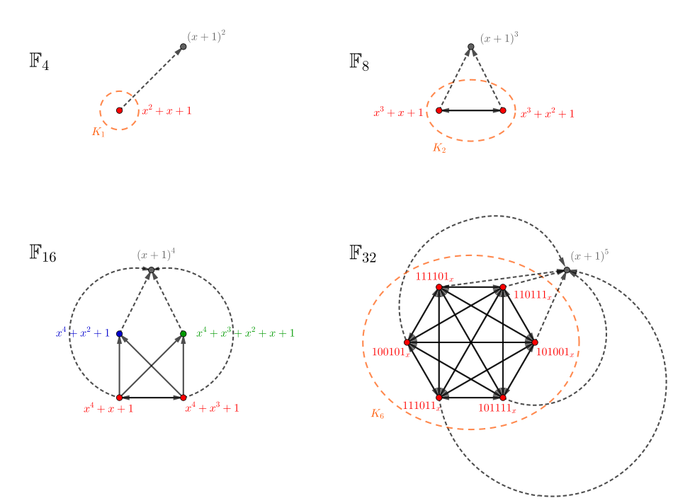
We can study the interplay of primitives, irreducibles, and their powers by converting our sequences into (directed) graphs. Each node in the graph will represent an irreducible polynomial over the field. Call the one under consideration a. If the sequence of characteristic polynomials generated by powers of Ca contains contains another polynomial b, then there is an edge from a to b.
-- Convert a polynomial to the integer representing it in characteristic nasPolyNum n = evalPoly n .fmap (`mod` n)irreducibleGraph d n =concatMap (\(x:xs) ->map (x,) xs) polyKinClasses where-- All irreducible polynomials of degree d in characteristic n irrsOfDegree' = irrsOfDegree d n-- Get "kin" polynomials as integers -- all those who appear as characteristic-- polynomials in the powers of its companion matrix getKinPolys =map (asPolyNum n . charpoly) . matrixPowersMod n . companion-- Kin classes corresponding to each irreducible polynomial,-- which is the first entry polyKinClasses =map (nub .take (n^d) . getKinPolys) irrsOfDegree'
We can do this for every GF(pm). Let’s start with the first few fields of characteristic 2. We get the following graphs:
All nodes connect to the node corresponding to the identity matrix, since all roots are cyclic. Also, since all primitive polynomials are interchangeable with one another, they are all interconnected and form a complete clique. This means that, excluding the identity node, the graphs for fields of order one more than a Mersenne prime are just the complete graphs.
Since all of the graphs share the identity node as a feature – a node with incoming edges from every other node – its convenient to omit it. Here are a few more of these graphs after doing so, over fields of other characteristics:
Code
-- Characteristic polynomial of the identity matrixeyePoly d n = asPolyNum n $ charpoly $ eye d-- Remove edges directed toward the characteristic polynomial of the identityirreducibleGraphNoEye d n =filter ((/=eyePoly d n) .snd) $ irreducibleGraph d n-- Only plot the graph for GF(9), since the others take too long to renderplotDigraph $ irreducibleGraphNoEye 23
GF(9)
GF(25)
GF(49)
GF(121)
GF(27)
GF(125)
GF(343)
Spectra
Again, since visually interpreting graphs is difficult, we can study an invariant. From these graphs of polynomials, we can compute their characteristic polynomials (to add another layer to this algebraic cake) and look at their spectra.
It turns out that a removing a fully-connected node (like the one for the identity matrix) has a simple effect on characteristic polynomial of a graph: it just removes a factor of x. Here are a few of the (identity-reduced) spectra, arranged into a table.
Code
-- Not technically correct, but enough for this exampleedgesToAdjacency [] = toMatrix [[0]]edgesToAdjacency es =Mat asArray where-- Vertices from the edge list vs = nub $ es >>= (\(x,y) -> [x,y])-- Lookup table for new vertices vs' =zip vs [0..]-- Largest vertex index for array bounds b =maximum$mapsnd vs'-- Lookup function for new edge reindexing lookupVs = fromJust .fliplookup vs'-- List of reindexed edges reindexed =map (bimap lookupVs lookupVs) es-- Use a list of 2-tuples to set addresses in a matrix to 1 asArray = listArray ((0,0),(b,b)) (repeat0) //map (, 1) reindexed-- Find roots of `p` by trial dividing the entries of `xs`findRootsFrom xs p =fmaphead$ partitionEithers $ recurse p xs where-- We only need to test roots we haven't failed to divide tails [] = [] tails x@(_:xs) = x:tails xs-- Try dividing `p` by every remaining 'integer' root from xs trialDivisions p xs =map (\x -> (x, p `synthDiv`Poly [-head x, 1])) $ tails xs-- Find the first root which has a zero remainder, or Nothing if none exists firstRoot p xs = listToMaybe $dropWhile ((/=0) .snd.snd) $ trialDivisions p xs-- We either found a root (r) and need to recurse with the quotient (q)-- Or we couldn't find a root, and terminate with the number of unfound roots recurse p xs =case firstRoot p xs of (Just (next@(r:_), (q,_))) ->Left r:recurse q next _ -> [Right$length (coeffs p) -1]-- Show the spectrumshowSpectrum (xs, y) = intercalate ", " showMults ++ showMissing where showMults =map showMult (rle Nothing xs)-- Markdown notation for a root x repeated y times showMult (x,y) =show x ++"^"++show y ++"^" showMissing =if y ==0then""else" "++show y ++" other roots"-- Run-length encode a list to a list containing (original entry, count) rle Nothing [] = [] rle (Just x) [] = [x] rle Nothing (x:xs) = rle (Just (x, 1)) xs rle (Just (y, c)) (x:xs)| x == y = rle (Just (y, c+1)) xs|otherwise= (y, c):rle (Just (x, 1)) xs-- Characteristic, degree, remarkdataCharGraphRow=CGR { cgrCharacteristic ::Int, cgrDegree ::Int, cgrRemark ::String }charGraphTable = columns (\(_, f) r -> f r) (\(c, _) ->Headed c) [ ("Characteristic", \(CGR n d _) ->if d ==2thenshow n else""), ("Order", show. \(CGR n d _) -> n^d), ("Spectrum", \(CGR n d _) -> showSpectrum $ findRootsFrom [-1..35] $ charpoly $fmapfromIntegral$ edgesToAdjacency $ irreducibleGraphNoEye d n), ("Remark", cgrRemark) ]markdown $ markdownTable charGraphTable [CGR22"",CGR23"Mersenne",CGR24"",CGR25"Mersenne",CGR32"",CGR33"Pseudo-Mersenne?",CGR52"",CGR53"Prime power in spectrum",CGR72"",CGR73"Composite in spectrum",CGR112"Composite in spectrum" ]
Characteristic
Order
Spectrum
Remark
2
4
01
8
-11, 11
Mersenne
16
-11, 02, 11
32
-15, 51
Mersenne
3
9
-11, 02, 11
27
-16, 01, 32
Pseudo-Mersenne?
5
25
-15, 05, 12, 31
125
-137, 03, 92, 191
Prime power in spectrum
7
49
-115, 06, 12, 32, 71
343
-1104, 05, 12, 52, 112, 352
Composite in spectrum
11
121
-143, 012, 12, 34, 72, 151
Composite in spectrum
Incredibly, all spectra shown are composed exclusively of integers, and thus, each of these graphs are integral graphs. Moreover, it does not appear that any integer sequences that one may try extracting from this table (for example, the multiplicity of -1) can be found in the Online Encyclopedia of Integer Sequences.
From what I was able to tell, the following subgraphs were also integral over the range I tested:
the induced subgraph of vertices corresponding to non-primitives
the complement of the previous graph with respect to the whole graph
the induced subgraph of vertices corresponding only to irreducibles
Unfortunately, proving any such relationship is out of the scope of this post (and my abilities).
Closing
This concludes the first foray into using matrices as elements of prime power fields. It is a subject which, using the tools of linear algebra, makes certain aspects of field theory more palatable and constructs some objects with fairly interesting properties.
One of the most intriguing parts to me is the sequence of polynomials generated by a companion matrix. Though I haven’t proven it, I suspect that it suffices to study only the sequence generated by a primitive polynomial. It seems to be possible to get the non-primitive sequences by looking at the subsequences where the indices are multiples of a factor of the length of the sequence. But this means that the entire story about polynomials and finite fields can be foregone entirely, and the problem instead becomes one of number theory.
This post has an addendum to it which discusses some additional notes about matrix roots and the Cayley-Hamilton theorem. The next post will focus on an “application” of matrix roots to other areas of abstract algebra. Diagrams made with Geogebra and NetworkX (GraphViz).
Footnotes
For finite fields, it might make sense to do the following procedure to generate every possible element:
Take all powers of a companion matrix C
Add all powers of C with prior elements of the field (times identity matrices)
Repeat until no new elements are generated
In fact, we can usually do a little better, as we’ll see.↩︎