Exploring Finite Fields, Part 3: Roll a d20

When we extend fields with matrices, what other structures do we encounter?

In the previous post, we focused on constructing finite fields using n×n matrices. These matrices came from from primitive polynomials of degree n over GF(p), and could be used to do explicit arithmetic over GF(pⁿ). In this post, we’ll look at a way to apply this in describing certain groups.

Weakening the Field

Recall the way we defined GF(4) in the first post. We took the irreducible polynomial p(x) = x² + x + 1, called its root α, and created addition and multiplication tables spanning the four elements. After the second post, we can do this more cleverly by mapping α to the companion matrix C_p over GF(2).

\begin{gather*} f : \mathbb{F_4} \longrightarrow \mathbb{F}_2 {}^{2 \times 2} \\[10pt] 0 \mapsto \left(\begin{matrix} 0 & 0 \\ 0 & 0 \end{matrix}\right) ~~ 1 \mapsto \left(\begin{matrix} 1 & 0 \\ 0 & 1 \end{matrix}\right) = I ~~ \alpha \mapsto \left(\begin{matrix} 0 & 1 \\ 1 & 1 \end{matrix}\right) = C_p \\ \\ \textcolor{red}{\alpha} + \textcolor{blue}{1} = \alpha^2 \mapsto \left(\begin{matrix} 1 & 1 \\ 1 & 0 \end{matrix}\right) = \textcolor{red} { \left(\begin{matrix} 0 & 1 \\ 1 & 1 \end{matrix}\right) } + \textcolor{blue}{ \left(\begin{matrix} 1 & 0 \\ 0 & 1 \end{matrix}\right) }\mod 2 \end{gather*}

In the images of f, the zero matrix has determinant 0 and all other elements have determinant 1. Therefore, the product of any two nonzero matrices always has determinant 1, and a nonzero determinant means the matrix is invertible. Per the definition of the field, the non-zero elements form a group with respect to multiplication. Here, they form a cyclic group of order 3, since C_p³ = I mod 2. This is also true using symbols, since α³ = 1.

Other Matrices

However, there are more 2×2 matrices over GF(2) than just these. There are two possible values in four locations, so there are 24 = 16 matrices, or 12 more than we’ve identified.

\begin{array}{c|c} \#\{a_{ij} = 1\} & \det = 0 & \det = 1 \\ \hline 1 & \scriptsize \left(\begin{matrix} 0 & 1 \\ 0 & 0 \end{matrix}\right) ~~ \left(\begin{matrix} 1 & 0 \\ 0 & 0 \end{matrix}\right) ~~ \left(\begin{matrix} 0 & 0 \\ 0 & 1 \end{matrix}\right) ~~ \left(\begin{matrix} 0 & 0 \\ 1 & 0 \end{matrix}\right) \\ 2 & \scriptsize \left(\begin{matrix} 1 & 1 \\ 0 & 0 \end{matrix}\right) ~~ \left(\begin{matrix} 0 & 0 \\ 1 & 1 \end{matrix}\right) ~~ \left(\begin{matrix} 0 & 1 \\ 0 & 1 \end{matrix}\right) ~~ \left(\begin{matrix} 1 & 1 \\ 0 & 0 \end{matrix}\right) & \scriptsize \textcolor{red}{ \left(\begin{matrix} 0 & 1 \\ 1 & 0 \end{matrix}\right) } \\ 3 & & \scriptsize \textcolor{red}{ \left(\begin{matrix} 1 & 1 \\ 0 & 1 \end{matrix}\right) } ~~ \textcolor{red}{ \left(\begin{matrix} 1 & 0 \\ 1 & 1 \end{matrix}\right) } \\ 4 & \scriptsize \left(\begin{matrix} 1 & 1 \\ 1 & 1 \end{matrix}\right) \end{array}

The matrices in the right column (in red) have determinant 1, which means they can also multiply with our field-like elements without producing a singular matrix. This forms a larger group, of which our field’s multiplication group is a subgroup. However, it is not commutative, since matrix multiplication is not commutative in general.

The group of all six matrices with nonzero determinant is called the general linear group of degree 2 over GF(2), written¹ GL(2, 2). We can sort the elements into classes by their order, or the number of times we have to multiply them before getting to the identity matrix (mod 2):

\begin{array}{} \text{Order 1} & \text{Order 2} & \text{Order 3} \\ \hline \left(\begin{matrix} 1 & 0 \\ 0 & 1 \end{matrix}\right) & \begin{align*} \left(\begin{matrix} 1 & 1 \\ 0 & 1 \end{matrix}\right) \\ \left(\begin{matrix} 1 & 0 \\ 1 & 1 \end{matrix}\right) \\ \left(\begin{matrix} 0 & 1 \\ 1 & 0 \end{matrix}\right) \end{align*} & \begin{align*} \left(\begin{matrix} 0 & 1 \\ 1 & 1 \end{matrix}\right) \\ \left(\begin{matrix} 1 & 1 \\ 1 & 0 \end{matrix}\right) \end{align*} \end{array}

If you’ve studied enough group theory, you know that there are two groups of order 6: the cyclic group of order 6, C₆, and the symmetric group on three elements, S₃. Since the former group has order-6 elements, but none of these matrices are of order 6, the matrix group must be isomorphic to the latter. Since the group is small, it’s not too difficult to construct an isomorphism between the two. Writing the elements of S₃ in cycle notation, we have:

\begin{gather*} e \mapsto \left(\begin{matrix} 1 & 0 \\ 0 & 1 \end{matrix}\right) \\ \\ (1 ~ 2) \mapsto \left(\begin{matrix} 1 & 1 \\ 0 & 1 \end{matrix}\right) \qquad (1 ~ 3) \mapsto \left(\begin{matrix} 1 & 0 \\ 1 & 1 \end{matrix}\right) \qquad (2 ~ 3) \mapsto \left(\begin{matrix} 0 & 1 \\ 1 & 0 \end{matrix}\right) \\ \\ (1 ~ 2 ~ 3) \mapsto \left(\begin{matrix} 0 & 1 \\ 1 & 1 \end{matrix}\right) \qquad (3 ~ 2 ~ 1) \mapsto \left(\begin{matrix} 1 & 1 \\ 1 & 0 \end{matrix}\right) \end{gather*}

Bigger Linear Groups

Of course, there is nothing special about GF(2) in this definition. For any field K, the general linear group GL(n, K) is composed of invertible n×n matrices under matrix multiplication.

For fields other than GF(2), a matrix can have a determinant other than 1. Since the determinant is multiplicative, the product of two determinant 1 matrices also has determinant 1. Therefore, the general linear group has a subgroup, the special linear group SL(n, K), consisting of these matrices.

Haskell implementation of GL and SL for prime fields

This implementation will be based on the Matrix type from the first post. Assume we have already defined matrix multiplication and addition.

import Data.Array (listArray, bounds, elems)
import Data.List (unfoldr)

-- Partition a list into lists of length n
reshape :: Int -> [a] -> [[a]]
reshape n = unfoldr (reshape' n) where
  reshape' n x = if null x then Nothing else Just $ splitAt n x

-- Convert list of lists to Matrix
-- Abuses listArray working across rows, then columns
toMatrix :: [[a]] -> Matrix a
toMatrix l = Mat $ listArray ((0,0),(n-1,m-1)) $ concat l where
  m = length $ head l
  n = length l

-- Convert Matrix to list of lists
fromMatrix :: Matrix a -> [[a]]
fromMatrix (Mat m) = let (_,(_,n)) = bounds m in reshape (n+1) $ elems m

With helper functions out of the way, we can move on to generating all matrices (mod n). Then, we filter for matrices with nonzero determinant (in the case of GL) and determinant 1 (in the case of SL).

import Control.Monad (replicateM)

-- All m x m matrices (mod n)
allMatrices :: Int -> Int -> [Matrix Int]
allMatrices m n = map toMatrix $ replicateM m vectors where
  -- Construct all vectors mod n using base-n expansions and padding
  vectors  = [pad $ coeffs $ asPoly n l | l <- [1..n^m-1]]
  -- Pad xs to length m with zero
  pad xs = xs ++ replicate (m - length xs) 0

-- All matrices, but paired with their determinants
matsWithDets :: Int -> Int -> [(Matrix Int, Int)]
matsWithDets m n = map (\x -> (x, determinant x `mod` n)) $ allMatrices m n

-- Nonzero determinants
mGL m n = map fst $ filter (\(x,d) -> d /= 0) $ matsWithDets m n
-- Determinant is 1
mSL m n = map fst $ filter (\(x,d) -> d == 1) $ matsWithDets m n

Projectivity

Another important matrix group is the projective general linear group, PGL(n, K). In this group, two matrices are considered equal if one is a scalar multiple of the other². Both this and the determinant 1 constraint can apply at the same time, forming the projective special linear group, PSL(n, K).

For GF(2), all of these groups are the same, since the only nonzero determinant and scalar multiple is 1. Therefore, it’s beneficial to contrast SL and PGL with another example.

Let’s arbitrarily examine GL(2, 5). Since 4 squares to 1 (mod 5) and we’re working with 2×2 matrices, the determinant is unchanged when a matrix is scalar-multiplied by 4. These multiples are identified in PSL. On the other hand, in PGL, there are classes of matrices with determinant 2 and 3, which do not square to 1. These classes are exactly the ones which are “left out” of PSL.

\begin{matrix} \boxed{ \begin{gather*} \large \text{GL}(2, 5) \\ \underset{\det = 4}{ \scriptsize \left(\begin{matrix} 0 & 1 \\ 1 & 1 \end{matrix} \right) }, \textcolor{red}{ \underset{\det = 1}{ \scriptsize \left(\begin{matrix} 0 & 2 \\ 2 & 2 \end{matrix} \right) }}, \underset{\det = 2}{ \scriptsize \left(\begin{matrix} 1 & 0 \\ 0 & 2 \end{matrix} \right) }, \underset{\det = 3}{ \scriptsize \left(\begin{matrix} 2 & 0 \\ 0 & 4 \end{matrix} \right) }, ... \end{gather*} } & \twoheadrightarrow & \boxed{ \begin{gather*} \large \text{PGL}(2,5) \\ \underset{\det = 1, ~4}{ \scriptsize \textcolor{red}{\left\{ \left(\begin{matrix} 0 & 1 \\ 1 & 1 \end{matrix} \right), \left(\begin{matrix} 0 & 2 \\ 2 & 2 \end{matrix} \right), ... \right\} }} \\ \underset{\det = 2, ~ 3}{ \scriptsize \left\{ \left(\begin{matrix} 1 & 0 \\ 0 & 2 \end{matrix} \right), \left(\begin{matrix} 2 & 0 \\ 0 & 4 \end{matrix} \right), ... \right\} } \\ ... \end{gather*} } \\ \\ \boxed{ \begin{gather*} \large \text{SL}(2,5) \\ \textcolor{red}{ \scriptsize \left(\begin{matrix} 0 & 2 \\ 2 & 2 \end{matrix} \right) }, \scriptsize \left(\begin{matrix} 0 & 3 \\ 3 & 3 \end{matrix} \right), ... \end{gather*} } & \twoheadrightarrow & \boxed{ \begin{gather*} \large \text{PSL}(2,5) \\ \textcolor{red}{ \left\{ \scriptsize \left(\begin{matrix} 0 & 2 \\ 2 & 2 \end{matrix} \right), \left(\begin{matrix} 0 & 3 \\ 3 & 3 \end{matrix} \right), ... \right\} } ... \end{gather*} } \end{matrix}

import Data.List (nubBy)

-- PGL and PSL require special equality.
-- It's certainly possible to write a definition which makes the classes explicit, as its own new type.
-- We could then define equality on this type through `Eq`.
-- This is rather inefficient, though, so I'll choose to work with the representatives instead.

-- Scalar-multiply a matrix (mod p)
scalarTimes :: Int -> Int -> Matrix Int -> Matrix Int
scalarTimes n k = fmap ((`mod` n) . (*k))

-- Construct all scalar multiples mod n, then check if ys is any of them.
-- This is ludicrously inefficient, and only works for fields.
projEq :: Int -> Matrix Int -> Matrix Int -> Bool
projEq n xs ys = ys `elem` [scalarTimes n k xs | k <- [1..n-1]]

-- Strip out duplicates in GL and SL with projective equality
mPGL m n = nubBy (projEq n) $ mGL m n
mPSL m n = nubBy (projEq n) $ mSL m n

Exceptional Isomorphisms

When K is a finite field, the smaller PSLs turn out specify some interesting groups. We’ve studied the case of PSL(2, 2) being isomorphic to S₃ already, but it is also the case that:

\begin{align*} &\text{PSL}(2,3) \cong A_4 & & \text{(order 24)} \\ \\ &\text{PSL}(2,4) \cong \text{PSL}(2,5) \cong A_5 & & \text{(order 60)} \\ \\ &\text{PSL}(2,7) \cong \text{PSL}(3,2) & & \text{(order 168)} \end{align*}

These relationships can be proven abstractly (and frequently are!). However, I always found myself wanting. For PSL(2, 3) and A₄, it’s trivial to assign elements to one another by hand. But A₅ is getting untenable, to say nothing of PSL(2, 7). In these circumstances, it’s a good idea to leverage the computer.

Warming Up: A₅ and PSL(2, 5)

A₅, the alternating group on 5 elements, is composed of the even permutations of 5 elements. It also happens to describe the rotations of an icosahedron. Within the group, there are three kinds of elements:

• The product of two 2-cycles, such as a = (1 2)(3 4)
  • On an icosahedron, this corresponds to a 180 degree rotation (or more precisely, 1/2 of a turn) about an edge
• 5-cycles, such as b = (1 2 3 4 5)
  • This corresponds to a 72 degree rotation (1/5 of a turn) around a vertex
• 3-cycles, such as ab = (2 4 5)
  • This corresponds to a 120 degree rotation (1/3 of a turn) around the center of a face

It happens to be the case that all elements of the group can be expressed as a product between a and b – they generate the group.

Mapping to Matrices

To create a correspondence with PSL(2, 5), we need to identify permutations with matrices. Obviously, the identity permutation goes to the identity matrix. Then, since a and b generate the group, we can search for two matrices which obey the same relations (under projective equality, since we’re working in PSL).

Fortunately, we have a computer, so we can search for candidates rather quickly. First, let’s note a matrix B which is cyclic of order 5 to correspond with b:

-- Repeatedly apply f to p, until the predicate z
-- (usually equality to some quantity) becomes True.
-- Get the length of the resulting list
orderWith :: Eq a => (a -> a -> a) -> (a -> Bool) -> a -> Int
orderWith f z p = (+1) $ length $ takeWhile (not . z) $ iterate (f p) p

-- Order with respect to PSL(2, 5): using matrix multiplication (mod 5)
-- and projective equality to the identity matrix
orderPSL25 = orderWith (\x -> fmap (`mod` 5) . (x |*|)) (projEq 5 $ eye 2)

-- Only order 5 elements of PSL(2, 5)
psl25_order5 = filter ((==5) . orderPSL25) $ mPSL 2 5

markdown $ ("$$B = " ++) $ (++ "... $$") $ intercalate " ~,~ " $
  take 5 $ map texifyMatrix psl25_order5

B = \left( \begin{matrix}2 & 0 \\ 1 & 2\end{matrix} \right) ~,~ \left( \begin{matrix}2 & 0 \\ 2 & 2\end{matrix} \right) ~,~ \left( \begin{matrix}2 & 0 \\ 3 & 2\end{matrix} \right) ~,~ \left( \begin{matrix}2 & 0 \\ 4 & 2\end{matrix} \right) ~,~ \left( \begin{matrix}0 & 1 \\ 1 & 1\end{matrix} \right)...

Arbitrarily, let’s pick the last entry on this list. Now, we can search for order-2 elements in PSL(2, 5) whose product with B has order 3. This matrix (A) matches exactly with a in A₅.

-- Start with B as a generator
psl25_gen_B = toMatrix [[0,2],[2,2]]

-- Only order 2 elements of PSL(2, 5)
psl25_order2 = filter ((==2) . orderPSL25) $ mPSL 2 5

-- Find an order 2 element whose product with `psl25_gen_B` has order 3
psl25_gen_A_candidates = filter ((==3) . orderPSL25 . (psl25_gen_B |*|))
  psl25_order2

markdown $ ("$$A = " ++) $ (++ "$$") $ intercalate " ~,~ " $
  map texifyMatrix psl25_gen_A_candidates

A = \left( \begin{matrix}1 & 0 \\ 0 & 4\end{matrix} \right) ~,~ \left( \begin{matrix}1 & 0 \\ 2 & 4\end{matrix} \right) ~,~ \left( \begin{matrix}2 & 1 \\ 2 & 3\end{matrix} \right) ~,~ \left( \begin{matrix}1 & 2 \\ 0 & 4\end{matrix} \right) ~,~ \left( \begin{matrix}2 & 2 \\ 1 & 3\end{matrix} \right)

Again, arbitrarily, we’ll pick the last entry from this list. Let’s also peek at what the matrix AB looks like.

psl25_gen_AB = (`mod` 5) <$> (psl25_gen_A_candidates !! 4) |*| psl25_gen_B

markdown $ ("$$" ++) $ (++ "$$") $ intercalate " \\quad " [
    "(AB) = " ++ texifyMatrix psl25_gen_AB,
    "(AB)^3 = " ++ texifyMatrix ((`mod` 5) <$> (psl25_gen_AB^3))
  ]

(AB) = \left( \begin{matrix}4 & 3 \\ 1 & 3\end{matrix} \right) \quad (AB)^3 = \left( \begin{matrix}2 & 0 \\ 0 & 2\end{matrix} \right)

We now have a correspondence between three elements of A₅ and PSL(2, 5). We can “run” both sets of the generators until we associate all elements to one another. This is most visually appealing to see as a Cayley graph³:

Cayley graph showing an isomorphism between A5 and PSL(2, 5).
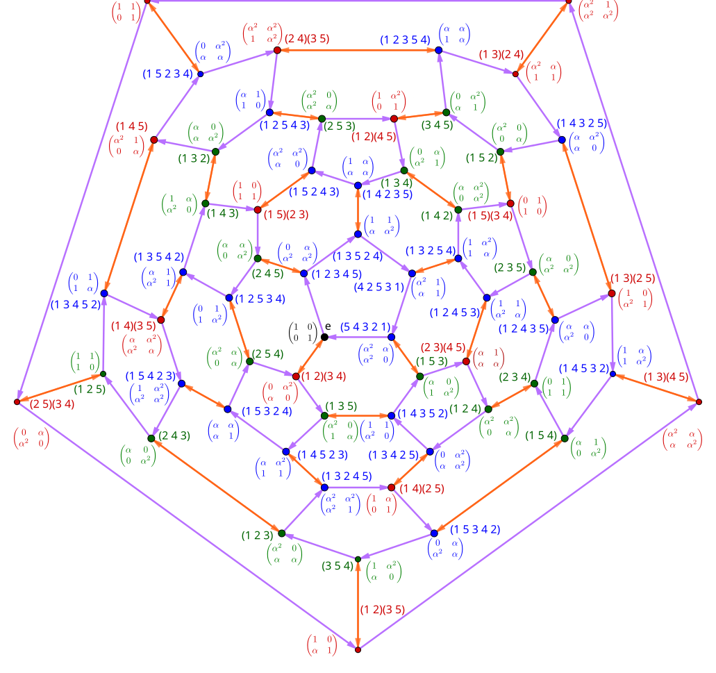
Order-2 elements are red, order-3 elements are green, and order-5 elements are blue. Purple arrows are order-5 generators, orange arrows are order-2 generators.

PSL(2, 4)

We could do the same for PSL(2, 4), but we can’t just work modulo 4 – remember, the elements of GF(4) are 0, 1, α, and α². It follows that GL(2, 4) is composed of (invertible) matrices of those elements, and SL(2, 4) is composed of matrices with determinant 1.

\begin{matrix} \boxed{ \begin{gather*} \large \text{GL}(2, 4) \\ \textcolor{red}{ \underset{\det = 1}{ \left(\begin{matrix} 0 & 1 \\ 1 & 1 \end{matrix} \right) }}, \underset{\det = \alpha + 1}{ \left(\begin{matrix} 0 & \alpha \\ \alpha & \alpha \end{matrix} \right) }, \underset{\det = \alpha}{ \left(\begin{matrix} 1 & 0 \\ 0 & \alpha \end{matrix} \right) }, \textcolor{red}{ \underset{\det = 1}{ \left(\begin{matrix} \alpha & 0 \\ 0 & \alpha^2 \end{matrix} \right) }}, ... \end{gather*} } \\ \\ \boxed{ \begin{gather*} \large \text{SL}(2,4) \\ \textcolor{red}{ \left(\begin{matrix} 0 & 1 \\ 1 & 1 \end{matrix} \right) }, \textcolor{red}{ \left(\begin{matrix} \alpha & 0 \\ 0 & \alpha^2 \end{matrix} \right) }, ... \end{gather*} } \end{matrix}

Scalar multiplication by α multiplies the determinant by α²; by α² multiplies the determinant by α⁴ = α. Thus, SL(2, 4) is also PSL(2, 4), since a scalar multiple has determinant 1.

Let’s start by looking at an order-5 matrix over PSL(2, 4). We’ll call this matrix B’ to correspond with our order-5 generator in PSL(2, 5).

\begin{gather*} B' = \left(\begin{matrix} 0 & \alpha \\ \alpha^2 & \alpha^2 \end{matrix} \right) \qquad (B')^2 = \left(\begin{matrix} 1 & 1 \\ \alpha & \alpha^2 \end{matrix}\right) \qquad (B')^3 = \left(\begin{matrix} \alpha^2 & 1 \\ \alpha & 1 \end{matrix}\right) \\ (B')^4 = \left(\begin{matrix} \alpha^2 & \alpha \\ \alpha^2 & 0 \end{matrix}\right) \qquad (B')^5 = \left(\begin{matrix} 1 & 0 \\ 0 & 1 \end{matrix}\right) \\ \\ \det B' = 0\alpha^2 - \alpha^3 = 1 \end{gather*}

We need to be able to do three things over GL(2, 4) on a computer:

• multiply matrices over GF(4),
• compute their determinant,
• visually distinguish between each of them, and
• be able to systematically write down all of them

It would then follow for us to repeat what we did with with SL(2, 5). But as I’ve said, working symbolically is hard for computers, and the methods described for prime fields do not work in general with prime power fields. Fortunately, we’re amply prepared to find a solution.

Bootstrapping Matrices

Recall that the elements of GF(4) can also be written as the zero matrix, the identity matrix, C_p, and C_p² (where C_p is the companion matrix of p(x) and again, p(x) = x² + x + 1). This means we can also write elements of GL(2, 4) as matrices of matrices. Arithmetic works exactly the same as it does symbolically – we just replace all instances of α in B’ with C_p.

\begin{gather*} f^* : \mathbb{F}_4 {}^{2 \times 2} \rightarrow (\mathbb{F}_2 {}^{2 \times 2})^{2 \times 2} \\ \\ \begin{align*} \bar {B'} = f^*(B') &= \left(\begin{matrix} f(0) & f(\alpha) \\ f(\alpha^2) & f(\alpha^2) \end{matrix} \right) = \left(\begin{matrix} {\bf 0} & C_p \\ C_p {}^2 & C_p {}^2 \end{matrix} \right) \\ &= \left(\begin{matrix} \left(\begin{matrix} 0 & 0 \\ 0 & 0 \end{matrix} \right) & \left(\begin{matrix} 0 & 1 \\ 1 & 1 \end{matrix} \right) \\ \left(\begin{matrix} 1 & 1 \\ 1 & 0 \end{matrix} \right) & \left(\begin{matrix} 1 & 1 \\ 1 & 0 \end{matrix} \right) \end{matrix} \right) \\ ~ \\ (f^*(\bar B'))^2 &= \left(\begin{matrix} ({\bf 0})({\bf 0}) + C_p {}^3 & ({\bf 0})C_p +C_p {}^3 \\ ({\bf 0})C_p {}^2 + C_p {}^4 & C_p {}^3 + C_p {}^4 \end{matrix} \right) \\ &= \left(\begin{matrix} I & I \\ C_p {} & C_p {}^2 \end{matrix} \right) = \left(\begin{matrix} f(1) & f(1) \\ f(\alpha) & f(\alpha^2) \end{matrix} \right) = f^*((B')^2) \end{align*} \end{gather*}

Make no mistake, this is not a block matrix, at least not a typical one. Namely, the layering means that the determinant (which signifies its membership in SL) is another matrix:

\begin{align*} \det( f^*(B') ) &= {\bf 0} (C_p {}^2) - (C_p)(C_p {}^2) \\ &= \left(\begin{matrix} 0 & 0 \\ 0 & 0 \end{matrix} \right) \left(\begin{matrix} 1 & 1 \\ 1 & 0 \end{matrix} \right) - \left(\begin{matrix} 0 & 1 \\ 1 & 1 \end{matrix} \right) \left(\begin{matrix} 1 & 1 \\ 1 & 0 \end{matrix} \right) \\ &= \left(\begin{matrix} 1 & 0 \\ 0 & 1 \end{matrix} \right) \mod 2 \\ &= I = f(\det(B')) \end{align*}

Since B’ is in SL(2, 4), the determinant is unsurprisingly f(1) = I. The (matrix) determinants of f* applied to other elements of GL(2, 4) could just as well be f(α) = C_p or f(α²) = C_p².

Implementation

Using this method, we can implement PSL(2, 4) directly. All we need to do is find all possible 4-tuples of 0, I, C_p, and C_p², then arrange each into a 2x2 matrix. Multiplication follows from the typical definition and the multiplicative identity is just f*(I).

import Data.List (elemIndex)

-- Matrices which obey the same relations as the elements of GF(4)
zero_f4 = zero 2
one_f4 = eye 2
alpha_f4 = toMatrix [[0,1],[1,1]]
alpha2_f4 = toMatrix [[1,1],[1,0]]

-- Gathered into a list
field4 = [zero_f4, one_f4, alpha_f4, alpha2_f4]

-- Convenient show function for these matrices
showF4 x = case elemIndex x field4 of
  Just 0 -> "0"
  Just 1 -> "1"
  Just 2 -> "α"
  Just 3 -> "α^2"
  Nothing -> "N/A"

-- Identity matrix over GF(4)
psl_24_identity = toMatrix [[one_f4, zero_f4], [zero_f4, one_f4]]

-- All possible matrices over GF(4)
-- Create a list of 4-lists of elements from GF(4), then
-- Shape them into 2x2 matrices
f4_matrices = map (toMatrix . reshape 2) $ replicateM 4 field4

-- Sieve out those which have a determinant of 1 in the field
mPSL24 = filter ((==one_f4) . fmap (`mod` 2) . laplaceDet) f4_matrices

Now that we can generate the group, we can finally repeat what we did with PSL(2, 5). All we have to do is filter out order-2 elements, then further filter for those which have an order-3 product with B’.

-- Order with respect to PSL(2, 4): using matrix multiplication (mod 2)
-- and projective equality to the identity matrix
orderPSL24 = orderWith (\x -> fmap (fmap (`mod` 2)) . (x*)) (== psl_24_identity)

-- Only order 2 elements of PSL(2, 4)
psl24_order2 = filter ((==2) . orderPSL24) mPSL24

-- Start with B as a generator
psl24_gen_B = toMatrix [[zero_f4, alpha_f4], [alpha2_f4, alpha2_f4]]

-- Find an order 2 element whose product with `psl24_gen_B` has order 3
psl24_gen_A_candidates = filter ((==3) . orderPSL24 . (psl24_gen_B |*|))
    psl24_order2

markdown $ ("$$ A' = " ++) $ (++ "$$") $ intercalate " ~,~ " $
  map (texifyMatrix' showF4) psl24_gen_A_candidates

A' = \left( \begin{matrix}0 & 1 \\ 1 & 0\end{matrix} \right) ~,~ \left( \begin{matrix}0 & α^2 \\ α & 0\end{matrix} \right) ~,~ \left( \begin{matrix}1 & 0 \\ 1 & 1\end{matrix} \right) ~,~ \left( \begin{matrix}1 & α^2 \\ 0 & 1\end{matrix} \right) ~,~ \left( \begin{matrix}α & 1 \\ α & α\end{matrix} \right)

We’ll pick the second entry as our choice of A’. We note that the product A’B’, does indeed have order 3.

psl24_gen_AB = fmap (`mod` 2) <$> (psl24_gen_A_candidates !! 1) |*| psl24_gen_B

markdown $ ("$$" ++) $ (++ "$$") $ intercalate " \\quad " [
    "(A'B') = " ++ texifyMatrix' showF4 psl24_gen_AB,
    "(A'B')^3 = " ++ texifyMatrix' showF4 (fmap (`mod` 2) <$> (psl24_gen_AB^3))
  ]

(A'B') = \left( \begin{matrix}α & α \\ 0 & α^2\end{matrix} \right) \quad (A'B')^3 = \left( \begin{matrix}1 & 0 \\ 0 & 1\end{matrix} \right)

Finally, we can arrange these matrices on a Cayley graph in the same way as PSL(2, 5):

Cayley graph showing an isomorphism between A₅ and PSL(2, 4).
Colors indicate the same thing as in the previous diagram.

Closing

This post addresses my original goal in implementing finite fields, namely computationally finding an explicit map between A₅ and PSL(2, 4). I believe the results are a little more satisfying than attempting to wrap your head around group-theoretic proofs. That’s not to discount the power and incredible logic that goes into the latter method. It does tend to leave things rather opaque, however.

If you’d prefer a more interactive diagram showing the above isomorphisms, I’ve gone to the liberty of creating a hoverable SVG:

Click to open interactive version

This post slightly diverts our course from the previous one’s focus on fields. The next one will focus on more results regarding the treatment of layered matrices. The algebraic consequences of this structure are notable in and of themselves, and are entirely obfuscated by the usual interpretation of block matrices.

Diagrams created with Geogebra and Inkscape.

Footnotes

1. Unfortunately, it’s rather easy to confuse “GF” with “GL”. Remember that “F” is for “field”, with the former standing for “Galois field”.

2. Equivalently, the elements are these equivalence classes. The product of two classes is the set of all possible products between the two classes, which is another class.

3. Different generators appear to be used for A and B due to some self-imposed turbulence when writing the original post. Under projective equality, both are the same as our choices of A and B.