Generating Polynomials, Part 1: Regular Constructibility
What kinds of regular polygons are constructible with compass and straightedge?
Recently, I used coordinate-free geometry to derive the volumes of the Platonic solids, a problem which was very accessible to the ancient Greeks. On the other hand, they found certain problems regarding which figures can be constructed via compass and straightedge to be very difficult. For example, they struggled with problems like doubling the cube or squaring the circle, which are known (through circa 19th century mathematics) to be impossible. However, before even extending planar geometry by a third dimension or calculating the areas of circles, a simpler problem becomes apparent. Namely, what kinds of regular polygons are constructible?
Regular Geometry and a Complex Series
When constructing a regular polygon, one wants a ratio between the length of a edge and the distance from a vertex to the center of the figure.
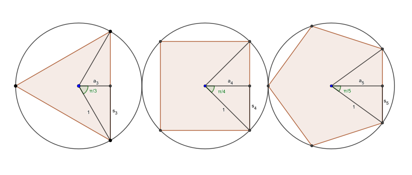
In a convex polygon, the total central angle is always one full turn, or 2π radians. The central angle of a regular n-gon is {2\pi \over n} radians, and the green angle above (which we’ll call θ) is half of that. This means that the ratio we’re looking for is \sin(\theta) = \sin(\pi / n). We can multiply by n inside the function on both sides to give \sin(n\theta) = \sin(\pi) = 0. Therefore, constructing a polygon is actually equivalent to solving this equation, and we can rephrase the question as how to express \sin(n\theta) (and \cos(n\theta)).
Complex Recursion
Thanks to Euler’s formula and de Moivre’s formula, the expressions we’re looking for can be phrased in terms of the complex exponential.
\begin{align*} e^{i\theta} &= \text{cis}(\theta) = \cos(\theta) + i\sin(\theta) & \text{ Euler's formula} \\ \text{cis}(n \theta) = e^{i(n\theta)} &= e^{(i\theta)n} = {(e^{i\theta})}^n = \text{cis}(\theta)^n \\ \cos(n \theta) + i\sin(n \theta) &= (\cos(\theta) + i\sin(\theta))^n & \text{ de Moivre's formula} \end{align*}
De Moivre’s formula for n = 2 gives
\begin{align*} \text{cis}(\theta)^2 &= (\text{c} + i\text{s})^2 \\ &= \text{c}^2 + 2i\text{cs} - \text{s}^2 + (0 = \text{c}^2 + \text{s}^2 - 1) \\ &= 2\text{c}^2 + 2i\text{cs} - 1 \\ &= 2\text{c}(\text{c} + i\text{s}) - 1 \\ &= 2\cos(\theta)\text{cis}(\theta) - 1 \end{align*}
This can easily be massaged into a recurrence relation.
\begin{align*} \text{cis}(\theta)^2 &= 2\cos(\theta)\text{cis}(\theta) - 1 \\ \text{cis}(\theta)^{n+2} &= 2\cos(\theta)\text{cis}(\theta)^{n+1} - \text{cis}(\theta)^n \\ \text{cis}((n+2)\theta) &= 2\cos(\theta)\text{cis}((n+1)\theta) - \text{cis}(n\theta) \end{align*}
Recurrence relations like this one are powerful. Through some fairly straightforward summatory manipulations, the sequence can be interpreted as the coefficients in a Taylor series, giving a generating function. Call this function F. Then,
\begin{align*} \sum_{n=0}^\infty \text{cis}((n+2)\theta)x^n &= 2\cos(\theta) \sum_{n=0}^\infty \text{cis}((n+1)\theta) x^n - \sum_{n=0}^\infty \text{cis}(n\theta) x^n \\ {F(x; \text{cis}(\theta)) - 1 - x\text{cis}(\theta) \over x^2} &= 2\cos(\theta) {F(x; \text{cis}(\theta)) - 1 \over x} - F(x; \text{cis}(\theta)) \\[10pt] F - 1 - x\text{cis}(\theta) &= 2\cos(\theta) x (F - 1) - x^2 F \\ F - 2\cos(\theta) x F + x^2 F &= 1 + x(\text{cis}(\theta) - 2\cos(\theta)) \\[10pt] F(x; \text{cis}(\theta)) &= {1 + x(\text{cis}(\theta) - 2\cos(\theta)) \over 1 - 2\cos(\theta)x + x^2} \end{align*}
Since \text{cis} is a complex function, we can separate F into real and imaginary parts. Conveniently, these correspond to \cos(n\theta) and \sin(n\theta), respectively.
\begin{align*} \Re[ F(x; \text{cis}(\theta)) ] &= {1 + x(\cos(\theta) - 2\cos(\theta)) \over 1 - 2\cos(\theta)x + x^2} \\ &= {1 - x\cos(\theta) \over 1 - 2\cos(\theta)x + x^2} = A(x; \cos(\theta)) \\ \Im[ F(x; \text{cis}(\theta)) ] &= {x \sin(\theta) \over 1 - 2\cos(\theta)x + x^2} = B(x; \cos(\theta))\sin(\theta) \end{align*}
In this form, it becomes obvious that the even though the generating function F was originally parametrized by \text{cis}(\theta), A and B are parametrized only by \cos(\theta). Extracting the coefficients of x yields an expression for \cos(n\theta) and \sin(n\theta) in terms of \cos(\theta) (and in the latter case, a common factor of \sin(\theta)).
If \cos(\theta) in A and B is replaced with the parameter z, then all trigonometric functions are removed from the equation, and we are left with only polynomials1. These polynomials are Chebyshev polynomials of the first (A) and second (B) kind. In actuality, the polynomials of the second kind are typically offset by 1 (the x in the numerator of B is omitted). However, retaining this term makes indexing consistent between A and B (and will make things clearer later).
We were primarily interested in \sin(n\theta), so let’s tabulate the first few polynomials of the second kind (at z / 2).
| n | [x^n]B(x; z / 2) = U_{n - 1}(z / 2) | Factored |
|---|---|---|
| 0 | 0 | 0 |
| 1 | 1 | 1 |
| 2 | z | z |
| 3 | z^{2} - 1 | \left(z - 1\right) \left(z + 1\right) |
| 4 | z^{3} - 2 z | z \left(z^{2} - 2\right) |
| 5 | z^{4} - 3 z^{2} + 1 | \left(z^{2} - z - 1\right) \left(z^{2} + z - 1\right) |
| 6 | z^{5} - 4 z^{3} + 3 z | z \left(z - 1\right) \left(z + 1\right) \left(z^{2} - 3\right) |
| 7 | z^{6} - 5 z^{4} + 6 z^{2} - 1 | \left(z^{3} - z^{2} - 2 z + 1\right) \left(z^{3} + z^{2} - 2 z - 1\right) |
| 8 | z^{7} - 6 z^{5} + 10 z^{3} - 4 z | z \left(z^{2} - 2\right) \left(z^{4} - 4 z^{2} + 2\right) |
| 9 | z^{8} - 7 z^{6} + 15 z^{4} - 10 z^{2} + 1 | \left(z - 1\right) \left(z + 1\right) \left(z^{3} - 3 z - 1\right) \left(z^{3} - 3 z + 1\right) |
| 10 | z^{9} - 8 z^{7} + 21 z^{5} - 20 z^{3} + 5 z | z \left(z^{2} - z - 1\right) \left(z^{2} + z - 1\right) \left(z^{4} - 5 z^{2} + 5\right) |
Evaluating the polynomials at z / 2 cancels the 2 in the denominator (and recurrence), making these expressions much simpler. This evaluation has an interpretation in terms of the previous diagram – recall we used half the length of a side as a leg of the right triangle. For a unit circumradius, the side length itself is then 2\sin( {\pi / n} ). To compensate for this doubling, the Chebyshev polynomial must be evaluated at half its normal argument.
Back on the Plane
The constructibility criterion is deeply connected to the Chebyshev polynomials. In compass and straightedge constructions, one only has access to linear forms (lines) and quadratic forms (circles). This means that a figure is constructible if and only if the root can be expressed using normal arithmetic (which is linear) and square roots (which are quadratic).
Pentagons
Let’s look at a regular pentagon. The relevant polynomial is
[x^5]B ( x; z / 2 ) = z^4 - 3z^2 + 1 = (z^2 - z - 1) (z^2 + z - 1)
According to how we derived this series, when z = 2\cos(\theta), the roots of this polynomial correspond to when \sin(5\theta) / \sin(\theta) = 0. This relation itself is true when \theta = \pi / 5, since \sin(5 \pi / 5) = 0.
One of the factors must therefore be the minimal polynomial of 2\cos(\pi / 5 ). The former happens to be correct correct, since 2\cos( \pi / 5 ) = \varphi, the golden ratio. Note that the second factor is the first evaluated at -z.
Heptagons
An example of where constructability fails is for 2\cos( \pi / 7 ).
\begin{align*} [x^7]B ( x; z / 2 ) &= z^6 - 5 z^4 + 6 z^2 - 1 \\ &= ( z^3 - z^2 - 2 z + 1 ) ( z^3 + z^2 - 2 z - 1 ) \end{align*}
Whichever is the minimal polynomial (the former), it is a cubic, and constructing a regular heptagon is equivalent to solving it for z. But there are no (nondegenerate) cubics that one can produce via compass and straightedge, and all constructions necessarily fail.
Decagons
One might think the same of 2\cos(\pi /10 )
\begin{align*} [x^{10}]B ( x; z / 2 ) &= z^9 - 8 z^7 + 21 z^5 - 20 z^3 + 5 z \\ &= z ( z^2 - z - 1 )( z^2 + z - 1 )( z^4 - 5 z^2 + 5 ) \end{align*}
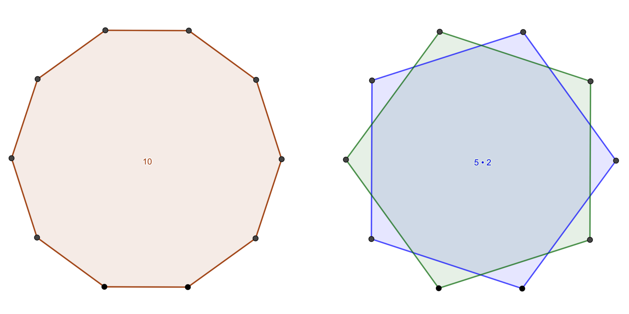
This expression also contains the polynomials for 2\cos( \pi / 5 ). This is because a regular decagon would contain two disjoint regular pentagons, produced by connecting every other vertex.
The polynomial which actually corresponds to 2\cos( \pi / 10 ) is the quartic, which seems to suggest that it will require a fourth root and somehow decagons are not constructible. However, it can be solved by completing the square…
\begin{align*} z^4 - 5z^2 &= -5 \\ z^4 - 5z^2 + (5/2)^2 &= -5 + (5/2)^2 \\ ( z^2 - 5/2)^2 &= {25 - 20 \over 4} \\ ( z^2 - 5/2) &= {\sqrt 5 \over 2} \\ z^2 &= {5 \over 2} + {\sqrt 5 \over 2} \\ z &= \sqrt{ {5 + \sqrt 5 \over 2} } \end{align*}
…and we can breathe a sigh of relief.
The Triangle behind Regular Polygons
Preferring z to be halved in B(x; z/2) makes something else more evident. Observe these four rows of the Chebyshev polynomials
| n | [x^n]B(x; z / 2) | k | [z^{k}][x^n]B(x; z / 2) |
|---|---|---|---|
| 4 | z^{3} - 2 z | 3 | 1 |
| 5 | z^{4} - 3 z^{2} + 1 | 2 | -3 |
| 6 | z^{5} - 4 z^{3} + 3 z | 1 | 3 |
| 7 | z^{6} - 5 z^{4} + 6 z^{2} - 1 | 0 | -1 |
The last column looks like an alternating row of Pascal’s triangle (namely, {n - \lfloor {k / 2} \rfloor - 1 \choose k}(-1)^k). This resemblance can be made more apparent by listing the coefficients of the polynomials in a table.
| n | z^9 | z^8 | z^7 | z^6 | z^5 | z^4 | z^3 | z^2 | z | 1 |
|---|---|---|---|---|---|---|---|---|---|---|
| 1 | 1 | |||||||||
| 2 | 1 | 0 | ||||||||
| 3 | 1 | 0 | -1 | |||||||
| 4 | 1 | 0 | -2 | 0 | ||||||
| 5 | 1 | 0 | -3 | 0 | 1 | |||||
| 6 | 1 | 0 | -4 | 0 | 3 | 0 | ||||
| 7 | 1 | 0 | -5 | 0 | 6 | 0 | -1 | |||
| 8 | 1 | 0 | -6 | 0 | 10 | 0 | -4 | 0 | ||
| 9 | 1 | 0 | -7 | 0 | 15 | 0 | -10 | 0 | 1 | |
| 10 | 1 | 0 | -8 | 0 | 21 | 0 | -20 | 0 | 5 | 0 |
Though they alternate in sign, the rows of Pascal’s triangle appear along diagonals, which I have marked in rainbow. Meanwhile, alternating versions of the naturals (1, 2, 3, 4…), the triangular numbers (1, 3, 6, 10…), the tetrahedral numbers (1, 4, 10, 20…), etc. are present along the columns, albeit spaced out by 0’s.
The relationship of the Chebyshev polynomials to the triangle is easier to see if the coefficient extraction of B(x; z / 2) is reversed. In other words, we extract z before extracting x.
\begin{align*} B(x; z / 2) &= {x \over 1 - zx + x^2} = {x \over 1 + x^2 - zx} = {x \over 1 + x^2} \cdot {1 \over {1 + x^2 \over 1 + x^2} - z{x \over 1 + x^2}} \\[10pt] [z^n]B(x; z / 2) &= {x \over 1 + x^2} [z^n] {1 \over 1 - z{x \over 1 + x^2}} = {x \over 1 + x^2} \left( {x \over 1 + x^2} \right)^n \\ &= \left( {x \over 1 + x^2} \right)^{n+1} = x^{n+1} (1 + x^2)^{-n - 1} \\ &= x^{n+1} \sum_{k=0}^\infty {-n - 1 \choose k}(x^2)^k \quad \text{Binomial theorem} \end{align*}
While the use of the binomial theorem is more than enough to justify the appearance of Pascal’s triangle (along with explaining the 0’s), I’ll simplify further to explicitly show the alternating signs.
\begin{align*} {(-n - 1)_k} &= (-n - 1)(-n - 2) \cdots (-n - k) \\ &= (-1)^k (n + k)(n + k - 1) \cdots (n + 1) \\ &= (-1)^k (n + k)_k \\ \implies {-n - 1 \choose k} &= {n + k \choose k}(-1)^k \\[10pt] [z^n]B(x; z / 2) &= x^{n+1} \sum_{k=0}^\infty {n + k \choose k} (-1)^k x^{2k} \end{align*}
Squinting hard enough, the binomial coefficient is similar to the earlier which gave the third row of Pascal’s triangle. If k is fixed, then this expression actually generates the antidiagonal entries of the coefficient table, which are the columns with uniform sign. The alternation instead occurs between antidiagonals (one is all positive, the next is 0’s, the next is all negative, etc.). The initial x^{n+1} lags these sequences so that they reproduce the triangle.
Imagined Transmutation
The generating function of the Chebyshev polynomials resembles other two term recurrences. For example, the Fibonacci numbers have generating function
\sum_{n = 0}^\infty \text{Fib}_n x^n = {1 \over 1 - x - x^2}
This resemblance can be made explicit with a simple algebraic manipulation.
\begin{align*} B(ix; -iz / 2) &= {1 \over 1 -\ (-i z)(ix) + (ix)^2} = {1 \over 1 -\ (-i^2) z x + (i^2)(x^2)} \\ &= {1 \over 1 -\ z x -\ x^2} \end{align*}
If z = 1, these two generating functions are equal. The same can be said for z = 2 with the generating function of the Pell numbers, and so on for higher recurrences (corresponding to metallic means) for higher integral z.
In terms of the Chebyshev polynomials, this series manipulation removes the alternation in the coefficients of U_n, restoring Pascal’s triangle to its nonalternating form. Related to the previous point, it is possible to find the Fibonacci numbers (Pell numbers, etc.) in Pascal’s triangle, which you can read more about here.
Manipulating the Series
Look back to the table of U_{n - 1}(z / 2) (Table 1). When I brought up U_{10 - 1}(z / 2) and decagons, I pointed out their relationship to pentagons as an explanation for why U_{5 -\ 1}(z / 2) appears as a factor. Conveniently, U_{2 -\ 1}(z / 2) = z is also a factor, and 2 is likewise a factor of 10.
This pattern is present throughout the table; n = 6 contains factors for n = 2 \text{ and } 3 and the prime numbers have no smaller factors. If this observation is legitimate, call the newest term f_n(z) and denote p_n(z) = U_{n -\ 1}( z / 2 ).
Factorization Attempts
The relationship between p_n and the intermediate f_d, where d is a divisor of n, can be made explicit by a Möbius inversion.
\begin{align*} p_n(z) &= \prod_{d|n} f_n(z) \\ \log( p_n(z) ) &= \log \left( \prod_{d|n} f_d(z) \right) = \sum_{d|n} \log( f_d(z) ) \\ \log( f_n(z) ) &= \sum_{d|n} { \mu \left({n \over d} \right)} \log( p_d(z) ) \\ f_n(z) &= \prod_{d|n} p_d(z)^{ \mu (n / d) } \\[10pt] f_6(z) = g_6(z) &= p_6(z)^{\mu(1)} p_3(z)^{\mu(2)} p_2(z)^{\mu(3)} \\ &= {p_6(z) \over p_3(z) p_2(z)} \end{align*}
Unfortunately, it’s difficult to apply this technique across our whole series. Möbius inversion over series typically uses more advanced generating functions such as Dirichlet series or Lambert series. However, naively reaching for these fails for two reasons:
- We built our series of polynomials on a recurrence relation, and these series are opaque to such manipulations.
- To do a proper Möbius inversion, we need these kinds of series over the logarithm of each polynomial (B is a series over the polynomials themselves).
Ignoring these (and if you’re in the mood for awful-looking math) you may note the Lambert equivalence2:
\begin{align*} \log( p_n(z) ) &= \sum_{d|n} \log( f_d(z) ) \\ \sum_{n = 1}^\infty \log( p_n ) x^n &= \sum_{n = 1}^\infty \sum_{d|n} \log( f_d ) x^n \\ &= \sum_{k = 1}^\infty \sum_{m = 1}^\infty \log( f_m ) x^{m k} \\ &= \sum_{m = 1}^\infty \log( f_m ) \sum_{k = 1}^\infty (x^m)^k \\ &= \sum_{m = 1}^\infty \log( f_m ) {x^m \over 1 - x^m} \end{align*}
Either way, the number-theoretic properties of this sequence are difficult to ascertain without advanced techniques. If research has been done, it is not easily available in the OEIS.
Total Degrees
It can be also be observed that the new term is symmetric (f(z) = f(-z)), and is therefore either irreducible or the product of polynomial and its reflection (potentially negated). For example,
p_9(z) = \left\{ \begin{matrix} (z - 1)(z + 1) & \cdot & (z^3 - 3z - 1)(z^3 - 3z + 1) \\ \shortparallel && \shortparallel \\ f_3(z) & \cdot & f_9(z) \\ \shortparallel && \shortparallel \\ g_3(z) \cdot g_3(-z) & \cdot & g_9(z) \cdot -g_9(-z) \end{matrix} \right.
These factor polynomials g_n are the minimal polynomials of 2\cos( \pi / n ).
Multiplying these minimal polynomials by their reflection can be observed in the Chebyshev polynomials for n = 3, 5, 7, 9, strongly implying that it occurs on the odd terms. Assuming this is true, we have
f_n(z) = \begin{cases} g_n(z) & \text{$n$ is even} \\ g_n(z)g_n(-z) & \text{$n$ is odd and ${\deg(f_n) \over 2}$ is even} \\ -g_n(z)g_n(-z) & \text{$n$ is odd and ${\deg(f_n) \over 2}$ is odd} \end{cases}
Without resorting to any advanced techniques, the degrees of f_n are not too difficult to work out. The degree of p_n(z) is n -\ 1, which is also the degree of f_n(z) if n is prime. If n is composite, then the degree of f_n(z) is n -\ 1 minus the degrees of the divisors of n -\ 1. This leaves behind how many numbers less than n are coprime to n. Therefore \deg(f_n) = \phi(n), the Euler totient function of the index.
The totient function can be used to examine the parity of n. If n is odd, it is coprime to 2 and all even numbers. The introduced factor of 2 to 2n removes the evens from the totient, but this is compensated by the addition of the odd multiples of old numbers coprime to n and new primes. This means that \phi(2n) = \phi(n) for odd n (other than 1).
The same argument can be used for even n: there are as many odd numbers from 0 to n as there are from n to 2n, and there are an equal number of numbers coprime to 2n in either interval. Therefore, \phi(2n) = 2\phi(n) for even n.
This collapses all cases of the conditional factorization of f_n into one, and the degrees of g_n are
\begin{align*} \deg( g_n(z) ) &= \begin{cases} \deg( f_n(z) ) = \phi(n) & n \text{ is even} & \implies \phi(n) = \phi(2n) / 2 \\ \deg( f_n(z) ) / 2 = \phi(n) / 2 & n \text{ is odd} & \implies \phi(n) / 2 = \phi(2n) / 2 \end{cases} \\ &= \varphi(2n) / 2 \end{align*}
Though they were present in the earlier Chebyshev table, the g_n themselves are presented again, along with the expression for their degree
| n | \varphi(2n)/2 | g_n(z) | Coefficient list, rising powers |
|---|---|---|---|
| 2 | 1 | z | [0, 1] |
| 3 | 1 | z - 1 | [-1, 1] |
| 4 | 2 | z^{2} - 2 | [-2, 0, 1] |
| 5 | 2 | z^{2} - z - 1 | [-1, -1, 1] |
| 6 | 2 | z^{2} - 3 | [-3, 0, 1] |
| 7 | 3 | z^{3} - z^{2} - 2 z + 1 | [1, -2, -1, 1] |
| 8 | 4 | z^{4} - 4 z^{2} + 2 | [2, 0, -4, 0, 1] |
| 9 | 3 | z^{3} - 3 z - 1 | [-1, -3, 0, 1] |
| 9 | 3 | z^{3} - 3 z + 1 | [1, -3, 0, 1] |
| 10 | 4 | z^{4} - 5 z^{2} + 5 | [5, 0, -5, 0, 1] |
| - | OEIS A055034 | - | OEIS A187360 |
Closing
My initial jumping off point for writing this article was completely different. However, in the process of writing, its share of the article shrank and shrank until its introduction was only vaguely related to what preceded it. But alas, the introduction via geometric constructions flows better coming off my post about the Platonic solids. Also, it reads better if I rely less on “if you search for this sequence of numbers” and more on how to interpret the definition.
Consider reading the follow-up to this post if you’re interested in another way one can obtain the Chebyshev polynomials. I have since rederived the Chebyshev polynomials without the complex exponential, which you can read about in this post.
Diagrams created with GeoGebra.
Footnotes
This can actually be observed as early as the recurrence relation.
\begin{align*} \text{cis}(\theta)^{n+2} &= 2\cos(\theta)\text{cis}(\theta)^{n+1} - \text{cis}(\theta)^n \\ a_{n+2} &= 2 z a_{n+1} - a_n \\ \Re[ a_0 ] &= 1,~~ \Im[ a_0 ] = 0 \\ \Re[ a_1 ] &= z,~~ \Im[ a_1 ] = 1 \cdot \sin(\theta) \end{align*} ↩︎
This equivalence applies to other polynomial series obeying the same factorization rule such as the cyclotomic polynomials.↩︎