Generating Polynomials, Part 2: Ghostly Chains
What do polygons without distance still know about planar geometry?
In the previous post, I tied the geometry regular polygons to a sequence of polynomials though some clever algebraic manipulation. But let’s deign to ask a very basic question: what is a polygon?
Loops without Distance
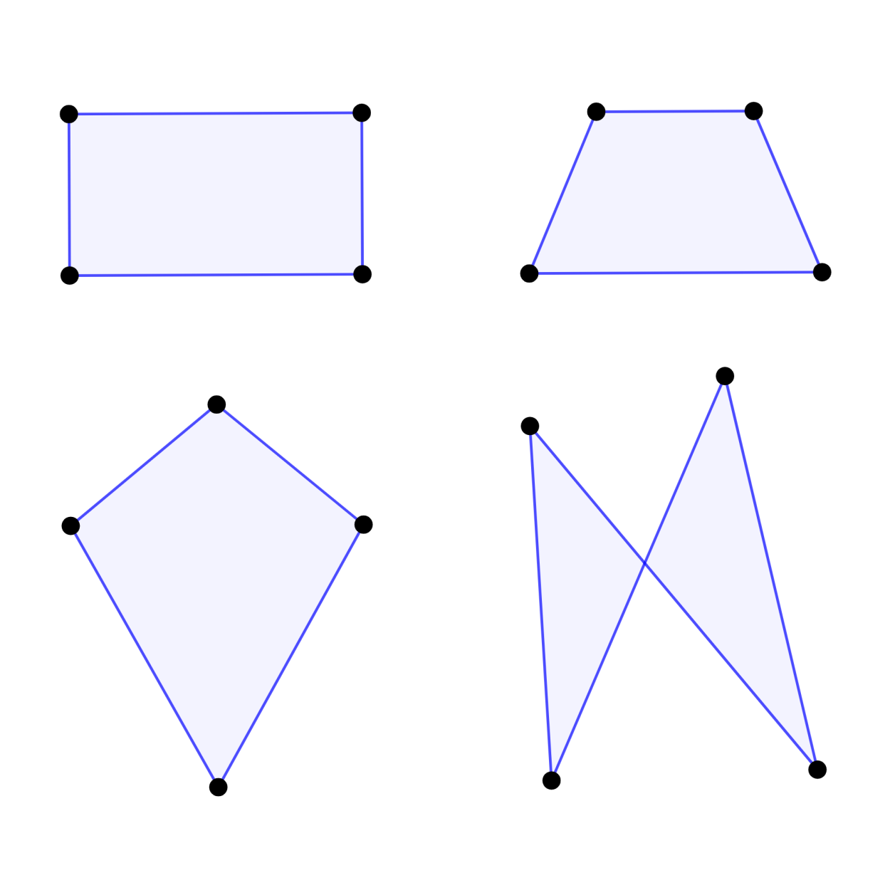
Fundamentally, a polygon is just a collection of vertices and edges. For polygons in a Euclidean setting, the position of points matters, as well as the lines connecting them – a rectangle is different from a trapezoid or a kite. But at its simplest, this is just a tabulation of points and adjacencies.
Only examining these figures by their connectedness is precisely the kind of thing graph theory deals with. “Graph” is a potentially confusing term, since it has nothing to do with “graphs of functions”, but the name is supposed to evoke the fact that they are “drawings”. For the graphs we’re interested in, there’s some additional terminology:
- Vertices themselves are sometimes instead called nodes
- Edge in the graph have no direction in how they connect nodes, so the graph is called undirected.
- If the nodes in a graph can be arranged so that no edges appear to intersect, the graph is planar.
- For example, lower-right figure in the above diagram appears to have intersecting edges, but the nodes can be rearranged to look like the other graphs, so it is planar.
It’s easiest to study families of graphs, rather than isolated examples. If the graph is a simple loop of nodes, it is called a cycle graph. They are denoted by C_n, where n is the number of nodes. In a cycle graph, since all nodes are identical to each other (they all connect to two edges) and all edges are identical to each other (they connect identical vertices), the best geometric interpretation is a shape which is
- Regular, so that each edge and each angle (vertex) are of equal measure
- Convex, so that no edge meets another without creating a vertex (or node)
In other words, C_3 is analogous to an equilateral triangle, C_4 is analogous to a square, and so on.
Encoding Graphs
There are two primary ways to store information about a graph. The first is by labelling each node (for example, with integers), then recording the edges as a list of pairs of connected nodes. In the case of an undirected graph, these are unordered pairs. While such a list is convenient, it doesn’t convey a lot of information about the graph besides the number of edges.
Alternatively, these pairs can also be interpreted as addresses in a square matrix, called an adjacency matrix. Each column and row correspond to a specific node, and an entry is 1 when the nodes of a row and column of are joined by an edge (and 0 otherwise). For undirected graphs, these matrices are symmetric, since it is possible to traverse an edge in either direction.
\begin{align*} C_3 := \begin{matrix}[ (0, 1), \\ (1, 2), \\ (2, 0) ]\end{matrix} & \cong \begin{pmatrix} 0 & 1 & 1 \\ 1 & 0 & 1 \\ 1 & 1 & 0 \end{pmatrix} \\ \\ C_4 := \begin{matrix} [ (0, 1), \\ (1, 2), \\ (2, 3), \\ (3, 0) ]\end{matrix} & \cong \begin{pmatrix} 0 & 1 & 0 & 1 \\ 1 & 0 & 1 & 0 \\ 0 & 1 & 0 & 1 \\ 1 & 0 & 1 & 0 \end{pmatrix} \\ \\ C_5 := \begin{matrix}[ (0, 1), \\ (1, 2), \\ (2, 3), \\ (3, 4), \\ (4, 0) ]\end{matrix} &\cong \begin{pmatrix} 0 & 1 & 0 & 0 & 1 \\ 1 & 0 & 1 & 0 & 0 \\ 0 & 1 & 0 & 1 & 0 \\ 0 & 0 & 1 & 0 & 1 \\ 1 & 0 & 0 & 1 & 0 \end{pmatrix} \end{align*}
Swapping the labels on two nodes is will exchange two rows and two columns of the adjacency matrix. Just one of these swaps would flip the sign of its determinant, but since they occur in pairs, the determinant is invariant of the labelling (equally, a graph invariant).
Prismatic Recurrence
The determinant of a matrix is also the product of its eigenvalues, which are another matrix invariant. The set of eigenvalues is also called its spectrum, and the study of the spectra of graphs is called spectral graph theory1,
Eigenvalues are the roots of the characteristic polynomial of a matrix. The matrix C_5 is sufficiently large enough to generalize to C_n, and its characteristic polynomial by Laplace expansion is:
\begin{gather*} Ax = \lambda x \implies (\lambda I - A)x = 0 \\ \\ c_5(\lambda) = |\lambda I - C_5| = \left | \begin{matrix} \lambda & -1 & 0 & 0 & -1 \\ -1 & \lambda & -1 & 0 & 0 \\ 0 & -1 & \lambda & -1 & 0 \\ 0 & 0 & -1 & \lambda & -1 \\ -1 & 0 & 0 & -1 & \lambda \end{matrix} \right | \\ = \lambda m_{1,1} + \overbrace{(-1)}^\text{entry}\overbrace{(-1)^{1 + 2 \ }}^\text{sign} m_{1, 2} + \overbrace{(-1)}^\text{entry}\overbrace{(-1)^{1 + 5 \ }}^\text{sign} m_{1, 5} \end{gather*}
Note that every occurrence of “5” generalizes to higher n. The first minor is easily expressed in terms of another matrix’s characteristic polynomial.
m_{1, 1}[C_5] = \left | \begin{matrix} \lambda & -1 & 0 & 0 \\ -1 & \lambda & -1 & 0 \\ 0 & -1 & \lambda & -1 \\ 0 & 0 & -1 & \lambda \end{matrix} \right | = |\lambda I - P_4| = p_{5 - 1}(\lambda)
We will come to the meaning of the P_n in a moment. The other minors require extra expansions, but ones that (thankfully) quickly terminate.
\begin{matrix} m_{1, 2}[C_5] &= \left | \begin{matrix} -1 & -1 & 0 & 0 \\ 0 & \lambda & -1 & 0 \\ 0 & -1 & \lambda & -1 \\ -1 & 0 & -1 & \lambda \end{matrix} \right | &=& (-1) \left | \begin{matrix} \lambda & -1 & 0 \\ -1 & \lambda & -1 \\ 0 & -1 & \lambda \end{matrix} \right | &+& (-1)(-1)^{1 + 4} \left | \begin{matrix} -1 & 0 & 0 \\ \lambda & -1 & 0 \\ -1 & \lambda & -1 \end{matrix} \right | \\ &&=& (-1)|\lambda I - P_3| &+& (-1)\overbrace{(-1)^{5}(-1)^{5 - 2}}^{\text{even power, even when $\scriptsize n \neq 5$}} \\ &&=& (-1)p_{5 - 2}(\lambda) &+& (-1) \\ &&=& -(p_{5 - 2}(\lambda) &+& 1) \end{matrix}
The “1 + 4” exponent when evaluating this minor comes from the address of the lower-left -1, (i.e., (1, 4)). This entry exists for all C_n. The determinant of the rightmost matrix is just the product of the -1’s on the diagonal, so it will always have a power of the same parity as n, which cancels out with the sign of the minor. Meanwhile, another P-type matrix appears in the other term, this time of two lower orders.
\begin{matrix} \\ \\ m_{1, 5}[C_5] &= \left | \begin{matrix} -1 & \lambda & -1 & 0 \\ 0 & -1 & \lambda & -1 \\ 0 & 0 & -1 & \lambda \\ -1 & 0 & 0 & -1 \end{matrix} \right | &=& (-1) \left | \begin{matrix} -1 & \lambda & -1 \\ 0 & -1 & \lambda \\ 0 & 0 & -1 \end{matrix} \right | &+& (-1)(-1)^{5 - 2} \left | \begin{matrix} \lambda & -1 & 0 \\ -1 & \lambda & -1 \\ 0 & -1 & \lambda \end{matrix} \right | \\ &&=& (-1)(-1)^{5-2} &+& (-1)(-1)^{5 - 2}|\lambda I - P_3| \\ &&=& (-1)^{5-1}((-1)(-1) &+& (-1)(-1)p_{5 - 2}(\lambda)) \\ &&=& (-1)^{5-1}(1 &+& p_{5 - 2}(\lambda)) \end{matrix}
A third P-type matrix appears, just like the other minor. Unfortunately, this minor does depend on the parity of n.
All together, this produces a characteristic polynomial in terms of the polynomials p_n(\lambda):
\begin{align*} && c_5(\lambda) &= \lambda p_{5 - 1} + (-1)(p_{5 - 2} + 1) + (-1)\overbrace{(-1)^{5 - 1} (-1)^{5 - 1}}^{\text{even, even when $\scriptsize n \neq 5$}}(p_{5 - 2} + 1) \\ &&&= \lambda p_{5 - 1} - (p_{5 - 2} + 1) - (p_{5 - 2} + 1) \\ &&&= \lambda p_{5 - 1} - 2(p_{5 - 2} + 1) \\ && \implies c_n(\lambda) &= \lambda p_{n - 1}(\lambda) - 2(p_{n - 2}(\lambda) + 1) \end{align*}
Fortunately, the minor whose determinant depended on the parity of n cancels with (-1)^{1 + 5}, and the resulting expression seems to generically apply across all n. Further, this resembles a recurrence relation, which is great for building a rule. But it is meaningless without knowing p_n(\lambda).
Powerful Chains
The various P_n are in fact the adjacency matrices of a path on n nodes.
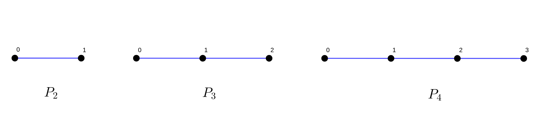
\begin{align*} P_2 &:= \begin{matrix}[ (0, 1) ]\end{matrix} \cong \begin{pmatrix} 0 & 1 \\ 1 & 0 \end{pmatrix} \\ P_3 &:= \begin{matrix}[ (0, 1), \\ (1, 2) ]\end{matrix} \cong \begin{pmatrix} 0 & 1 & 0 \\ 1 & 0 & 1 \\ 0 & 1 & 0 \end{pmatrix} \\ P_4 &:= \begin{matrix}[ (0, 1), \\ (1, 2), \\ (2, 3) ]\end{matrix} \cong \begin{pmatrix} 0 & 1 & 0 & 0 \\ 1 & 0 & 1 & 0 \\ 0 & 1 & 0 & 1 \\ 0 & 0 & 1 & 0 \end{pmatrix} \end{align*}
These matrices are similar to the ones for cycle graphs, but lack the entries in bottom-left and upper-right corners. Consequently, the characteristic polynomials of P_n are much easier to solve for.
\begin{gather*} p_4(\lambda) = |\lambda I - P_4| = \left | \begin{matrix} \lambda & -1 & 0 & 0 \\ -1 & \lambda & -1 & 0 \\ 0 & -1 & \lambda & -1 \\ 0 & 0 & -1 & \lambda \end{matrix} \right | \\ \\ = \lambda \left | \begin{matrix} \lambda & -1 & 0 \\ -1 & \lambda & -1 \\ 0 & -1 & \lambda \end{matrix} \right | + (-1)(-1)^{1+2} \left | \begin{matrix} -1 & -1 & 0 \\ 0 & \lambda & -1 \\ 0 & -1 & \lambda \end{matrix} \right | \\ \\ = \lambda |\lambda I - P_3| + \left ( (-1) \left | \begin{matrix} \lambda & -1 \\ -1 & \lambda \end{matrix} \right | + (-1)(-1) \left | \begin{matrix} 0 & -1 \\ 0 & \lambda \end{matrix} \right | \right) \\ \\ = \lambda |\lambda I - P_3| - |\lambda I - P_2| \\ = \lambda p_{4 - 1}(\lambda) - p_{4 - 2}(\lambda) \\ \implies p_{n}(\lambda) = \lambda p_{n - 1}(\lambda) - p_{n - 2}(\lambda) \end{gather*}
While the earlier equation for c_n in terms of p_n reminded of a recurrence relation, this actually is one (and it should look familiar).
Since the recurrence has order 2, it requires two initial terms: p_0 and p_1. The graph corresponding to p_1 is a single node, not connected to anything. Therefore, its adjacency matrix is a 1x1 matrix with 0 as its only entry, and its characteristic polynomial is \lambda. By the recurrence, p_2 = \lambda p_1 -\ p_0 = \lambda^2 -\ p_0. Equating terms with the characteristic polynomial of P_2, it is obvious that
|\lambda I - P_2| = \begin{pmatrix} \lambda & -1 \\ -1 & \lambda \end{pmatrix} = \lambda^2 - 1 = \lambda p_1 - p_0 \\ \implies p_0 = 1
which makes sense, since p_0 should have degree zero. Therefore, the sequence of polynomials p_n(\lambda) is:
\begin{gather*} p_0(\lambda) &=&& && 1 \\ p_1(\lambda) &=&& && \lambda \\ p_2(\lambda) &=&& \lambda \lambda - 1 &=& \lambda^2 - 1 \\ p_3(\lambda) &=&& \lambda (\lambda^2 - 1) - \lambda &=& \lambda(\lambda^2 - 2) \\ p_4(\lambda) &=&& \lambda (\lambda(\lambda^2 - 2)) - (\lambda^2 - 1) &=& \lambda^4 - 3\lambda^2 + 1 \\ \vdots & && \vdots && \vdots \end{gather*}
But wait, we’ve seen these before (if you read the previous post, that is). These are just the Chebyshev polynomials of the second kind, evaluated at \lambda / 2. Indeed, their recurrence relations are identical, so the characteristic polynomial of P_n is U_n(\lambda / 2). Effectively, this connects an n-path to a regular n+1-gon.
Back to Cycles
Since the generating function of U_n is known, the generating function for the c_n (which prompted this) is also easily determined. For ease of use, let
P(x; \lambda) = {B(x; \lambda / 2) \over x} = {1 \over 1 - \lambda x +\ x^2}
Discarding the initial c_0 and c_1 by setting them to zero2, the generating function is
\begin{align*} c_{n+2}(\lambda) &= \lambda p_{n+1}(\lambda) - 2(p_n(\lambda) + 1) \\[14pt] {C(x; \lambda) - c_0(\lambda) - x c_1(\lambda) \over x^2} &= \lambda \left( {P(x; \lambda) - 1 \over x} \right) - 2\left( P(x; \lambda) + {1 \over 1 - x} \right) \\ C &= x \lambda (P - 1) -\ 2x^2\left( P + {1 \over 1 - x} \right) \\ C{(1 - x) \over P} &= x \lambda \left(1 - {1 \over P} \right)(1 - x) -\ 2x^2\left( (1 - x) + {1 \over P} \right) \\ &= x^4 \lambda - 2 x^4 - x^3 \lambda^2 + x^3 \lambda + 2 x^3 + x^2 \lambda^2 - 4 x^2 \\ &= x^2 (\lambda - 2) (x^2 - \lambda x - x + \lambda + 2) \\[14pt] C(x; \lambda) &= x^2 (\lambda - 2) {(x^2 - (\lambda + 1) x + \lambda + 2) \over (1 - x)(1 - \lambda x + x^2)} \end{align*}
While the numerator is considerably more complicated than the one for P, the factor \lambda - 2 drops out of the entire series. This pleasantly informs that 2 is an eigenvalue of all C_n.
Off the Beaten Path
When we use Laplace expansion on the adjacency matrices, we were very fortunate that the minors also looked like adjacency matrices undergoing expansion. This let us terminate early and recurse. From the perspective of the graph, Laplace expansion almost looks like removing a node, but requires special treatment for the nodes connected to the one being removed. For example, in cycle graphs, the first stage of expansion had three minors:
- The node itself, on the main diagonal
- Being on the main diagonal, this immediately produced another adjacency matrix.
- Either neighbor connected to it, which are on opposite sides of a path after the node is removed
- Both of these nodes required second expansion to get the λs back on the main diagonal.
For “good enough” graphs that are nearly paths (including paths themselves), this gives a second-order recurrence relation.
Trees
Another simple family of graphs are trees. In some sense, they are the opposite of cycle graphs, since by definition they contain no cycles.
Paths are degenerate trees, but we can make them slightly more interesting by instead adding exactly one node and edge to (the middle of) a path.

In this notation, the subscripts denote the consituent paths if the “added” node and the one it is connected to are both removed. It’s easy to see that T_{a,b} \cong T_{a,b}, since this just swaps the arms. Also, T_{a, 0} \cong T_{0, a} \cong P_{a + 2}.
Let’s try dissecting some of the larger trees. The adjacency matrices for T_{1,3} and T_{2,2} are:
\begin{align*} T_{1,3} := \begin{matrix}[ (0, 1), \\ (1, 2), \\ (2, 3), \\ (3, 4), \\ (1, 5) ]\end{matrix} &\cong \begin{pmatrix} 0 & 1 & 0 & 0 & 0 & 0 \\ 1 & 0 & 1 & 0 & 0 & 1 \\ 0 & 1 & 0 & 1 & 0 & 0 \\ 0 & 0 & 1 & 0 & 1 & 0 \\ 0 & 0 & 0 & 1 & 0 & 0 \\ 0 & 1 & 0 & 0 & 0 & 0 \end{pmatrix} \\ \\ T_{2,2} := \begin{matrix}[ (0, 1), \\ (1, 2), \\ (2, 3), \\ (3, 4), \\ (2, 5) ]\end{matrix} &\cong \begin{pmatrix} 0 & 1 & 0 & 0 & 0 & 0 \\ 1 & 0 & 1 & 0 & 0 & 0 \\ 0 & 1 & 0 & 1 & 0 & 1 \\ 0 & 0 & 1 & 0 & 1 & 0 \\ 0 & 0 & 0 & 1 & 0 & 0 \\ 0 & 0 & 1 & 0 & 0 & 0 \end{pmatrix} \end{align*}
Starting with T_{1,3}, its characteristic polynomial is:
\begin{align*} |I \lambda - T_{1,3}| &= \left | \begin{matrix} \lambda & -1 & 0 & 0 & 0 & 0 \\ -1 & \lambda & -1 & 0 & 0 & -1 \\ 0 & -1 & \lambda & -1 & 0 & 0 \\ 0 & 0 & -1 & \lambda & -1 & 0 \\ 0 & 0 & 0 & -1 & \lambda & 0 \\ 0 & -1 & 0 & 0 & 0 & \lambda \end{matrix} \right | \\ &= \lambda (-1)^{6 + 6} m_{6,6} + (-1) (-1)^{2 + 6} m_{2,6} \end{align*}
It’s easy to see that m_{6,6} is just p_5(\lambda), since the rest of the graph other than the additional node is a 5-path. But the other minor is trickier.
\begin{align*} m_{2,6} &= \left | \begin{matrix} \lambda & -1 & 0 & 0 & 0 \\ 0 & -1 & \lambda & -1 & 0 \\ 0 & 0 & -1 & \lambda & -1 \\ 0 & 0 & 0 & -1 & \lambda \\ 0 & -1 & 0 & 0 & 0 \end{matrix} \right | \\ &= (-1) (-1)^{5 + 2} \left | \begin{matrix} \lambda & 0 & 0 & 0 \\ 0 & \lambda & -1 & 0 \\ 0 & -1 & \lambda & -1 \\ 0 & 0 & -1 & \lambda \\ \end{matrix} \right | \end{align*}
Through one extra expansion, the determinant of this final matrix can be written as a product of \lambda and p_3(\lambda).
Before making any conjectures, let’s do the same thing to T_{2,2}.
\begin{align*} |I \lambda - T_{2,2}| &= \left | \begin{matrix} \lambda & -1 & 0 & 0 & 0 & 0 \\ -1 & \lambda & -1 & 0 & 0 & 0 \\ 0 & -1 & \lambda & -1 & 0 & -1 \\ 0 & 0 & -1 & \lambda & -1 & 0 \\ 0 & 0 & 0 & -1 & \lambda & 0 \\ 0 & 0 & -1 & 0 & 0 & \lambda \end{matrix} \right | \\ &= (-1)^{6 + 6} \lambda m_{6,6} + (-1) (-1)^{3 + 6} m_{3,6} \\ \\ m_{3,6} &= \left | \begin{matrix} \lambda & -1 & 0 & 0 & 0 \\ -1 & \lambda & -1 & 0 & 0 \\ 0 & 0 & -1 & \lambda & -1 \\ 0 & 0 & 0 & -1 & \lambda \\ 0 & 0 & -1 & 0 & 0 \end{matrix} \right | \\ &= (-1) (-1)^{5 + 3} \left | \begin{matrix} \lambda & -1 & 0 & 0 \\ -1 & \lambda & 0 & 0 \\ 0 & 0 & \lambda & -1 \\ 0 & 0 & -1 & \lambda \\ \end{matrix} \right | \end{align*}
Here we get something similar: a combination of p_5(\lambda) and an extra term. In this case, the final determinant can be written as p_2(\lambda)^2.
Now it can be observed that the extra terms are the polynomials corresponding to P_a and P_b (recall that p_1(\lambda) = \lambda, after all). In both cases, the second expansion was necessary to get rid of the symmetric -1 entries added to the matrix. The sign of this extra term is always negative, since the -1 entries cancel and one of the signs of the minors along the two expansions must be negative.
Therefore, the expression for these characteristic polynomials should be:
t_{a,b}(\lambda) = \lambda p_{a + b + 1}(\lambda) - p_a(z) p_b(\lambda)
Note that if b is 0, this agrees with the recurrence for p_n(\lambda).
Examining Small Trees
Due to the subscript of the first term of the RHS, this recurrence is harder to turn into a generating function. Instead, let’s look at a few smaller trees to see what kind of polynomials they build. We’ll also change the variable of the polynomial to z for simplicity.
The first tree of note is T_{1,1}. This has characteristic polynomial
\begin{align*} t_{1,1}(z) &= z p_{3}(z) - p_1(z) p_1(z) \\ &= z (z^3 - z^2) - z^2 \\ &= z^2 (z^2 - 3) \end{align*}
Next, we have both T_{2,1} and T_{1,2}. By symmetry, these are the same graph, so we have characteristic polynomial
\begin{align*} t_{1,2}(z) &= z p_{4}(z) - p_1(z) p_2(z) \\ &= z (z^4 - 3z^2 + 2) - z \cdot (z^2 - 1) \\ &= z (z^4 - 4z^2 + 2) \end{align*}
Finally, let’s look at T_{1,3} and T_{2,2}, the trees we used to derive the rule.
\begin{align*} t_{1,3}(z) &= z p_{5}(z) - p_1(z) p_3(z) \\ &= z (z^5 - 4z^3 + 3z) - z \cdot (z^3 - 2z) \\ &= z^2 (z^4 - 5z^2 + 5) \\[10pt] t_{2,2}(z) &= z p_{5}(z) - p_2(z) p_2(z) \\ &= z (z^5 - 4z^3 + 3z) - ( z^2 - 1 )^2 \\ &= (z^2 - 1)(z^4 - 4z^2 + 1) \end{align*}
Many of these expressions factor surprisingly nicely. Further, some of these might seem familiar. From the last post, we saw that z^4 - 5z^2 + 5 is a factor of p_9(z), from which we know it is the minimal polynomial of 2 \cos(\pi / 10).
This is also true for:
- In t_{1,2}, the factor z^4 - 4z^2 + 2, p_7(z), and 2 \cos(\pi / 8), respectively
- In t_{2,2}, the factor z^4 - 4z^2 + 1, p_11(z), and 2 \cos(\pi / 12), respectively
We established that the subscripts of the tree (a and b) indicate constituent n-paths, which we know to correspond to n+1-gons. But these trees also seem to “know” about higher polygons.
Some Extra Trees
T_{2,3} is the first tree not to partition two equal paths or a path and a single node. In this regard, the next such tree is T_{2,4}.
These graphs turn out to have characteristic polynomials whose factors we haven’t seen before.
\begin{align*} t_{2,3}(z) &= z (z^{6} - 6 z^{4} + 9 z^{2} - 3) \\ t_{2,4}(z) &= z^{8} - 7 z^{6} + 14 z^{4} - 8 z^{2} + 1 \end{align*}
Searching the OEIS for the coefficients of t_{2,4} returns sequence A228786, which informs that it is the minimal polynomial of 2\sin( \pi/15 ). This sequence also informs that the unknown factor in the other polynomial is the minimal polynomial of 2\sin( \pi / 9 ):
In fact, both of these polynomials show up in factorizations of Chebyshev polynomials of the first kind (specifically, 2T_15(z / 2) and 2T_9(z / 2)). Perhaps this is not surprising since we were already working with those of the second kind. However, it is interesting to see them appear from the addition of a single node.
Closing
Regardless of whether chains or polygons are more fundamental, it is certainly interesting that they are just an algebraic stone’s (a calculus’s?) toss away from one another. Perhaps Euler skipped such stones from the bridges of Koenigsberg which inspired him to initiate graph theory.
Trees are certainly more complicated than either, and we only investigated those removed from a path by a single node. Regardless, they still related to Chebyshev polynomials, albeit through their factors.
In fact, I was initially prompted to look into them due to a remarkable correspondence between certain trees and Platonic solids. I have since reorganized these thoughts, as from the perspective of this article, the relationship is tangential at best.