Numbering Numbers: From 0 to ∞

How do we count an infinitude of numbers?

The infinite is replete with paradoxes. Some of the best come from comparing sizes of infinite collections. For example, every natural number can be mapped to a (nonnegative) even number and vice versa.

\begin{gather*} \N \rightarrow 2\N \\ n \mapsto 2n \\ \\ 0 \mapsto 0,~ 1 \mapsto2,~ 2 \mapsto 4,~ 3 \mapsto 6,~ 4 \mapsto 8, ... \end{gather*}

(For the purposes of this post, 0 \in \N, ~ 0 \notin \N^+)

All even numbers are “hit” by this map (by the definition of an even number), and no two natural numbers map to the same even number (again, more or less by definition, since 2m = 2n implies that m = n over \N). Therefore, the map is one-to-one and onto, so the map is a bijection. A consequence is that the map has an inverse, namely by reversing all of the arrows in the above block (i.e., the action of halving an even number).

Bijections with the natural numbers are easier to understand as a way to place things into a linear sequence. In other words, they enumerate “some sort of item”; in this case, even numbers.

In the finite world, a bijection between two things implies that they have the same size. It makes sense to extend the same logic to the infinite world, but there’s a catch. The nonnegative even numbers are clearly a strict subset of the natural numbers, but by this argument they have the same size.

\begin{matrix} 2\N & \longleftrightarrow & \N & \hookleftarrow & 2\N \\ 0 & \mapsto & \textcolor{red}0 & \dashleftarrow & \textcolor{red}0 \\ 2 & \mapsto & 1 & & \\ 4 & \mapsto & \textcolor{red}2 & \dashleftarrow & \textcolor{red}2 \\ 6 & \mapsto & 3 & & \\ 8 & \mapsto & \textcolor{red}4 & \dashleftarrow & \textcolor{red}4 \\ 10 & \mapsto & 5 & & \\ 12 & \mapsto & \textcolor{red}6 & \dashleftarrow & \textcolor{red}6 \\ 14 & \mapsto & 7 & & \\ 16 & \mapsto & \textcolor{red}8 & \dashleftarrow & \textcolor{red}8 \\ \vdots & & \vdots & & \vdots \end{matrix}

Are we Positive?

The confusion continues if we look at the integers and the naturals. Integers are the natural numbers and their negatives, so it would be intuitive to assume that there are twice as many of them as there are naturals (more or less one to account for zero). But since that logic fails for the naturals and the even numbers, it fails for the naturals and integers as well.

\begin{gather*} \begin{align*} \mathbb{N} &\rightarrow \mathbb{Z} \\ n &\mapsto \left\{ \begin{matrix} n/2 & n \text{ even} \\ -(n+1)/2 & n \text{ odd} \end{matrix} \right. \end{align*} \\ \\ 0 \mapsto 0,\quad 2 \mapsto 1, \quad 4 \mapsto 2, \quad 6 \mapsto 3, \quad 8 \mapsto 4,~... \\ 1 \mapsto -1, \quad 3 \mapsto -2, \quad 5 \mapsto -3, \quad 7 \mapsto -4, \quad 9 \mapsto -5,~... \end{gather*}

Or, in Haskell¹:

type Nat = Int

listIntegers :: Nat -> Int
listIntegers n
  | n < 0     = undefined
  | even n    = n `div` 2
  | otherwise = -(n + 1) `div` 2

In other words, this map sends even numbers to the naturals (the inverse of the doubling map) and the odds to the negatives. The same arguments about the bijective nature of this map apply as before, and so the paradox persists, since naturals are also a strict subset of integers.

Rational Numbers

Rationals are a bit worse. To make things a little easier, let’s focus on the positive rationals (i.e., fractions excluding 0). Unlike the integers, there is no obvious “next rational” after (or even before) 1. If there were, we could follow it with its reciprocal, like how an integer is followed by its negative in the map above.

On the other hand, the integers provide a sliver of hope that listing all rational numbers is possible. Integers can be defined as pairs of natural numbers, along with a way of considering two pairs equal.

\begin{gather*} -1 = (0,1) \sim_\Z (1,2) \sim_\Z (2,3) \sim_\Z (3,4) \sim_\Z ... \\[10pt] (a,b) \sim_\mathbb{Z} (c,d) \iff a+d = b+c \quad a,b,c,d \in \mathbb{N} \\[10pt] \mathbb{Z} := ( \mathbb{N} \times \mathbb{N} ) / \sim_\mathbb{Z} \end{gather*}

intEqual :: (Nat, Nat) -> (Nat, Nat) -> Bool
intEqual (a, b) (c, d) = a + d == b + c

This relation is the same as saying a - b = c - d (i.e., that -1 = 0 - 1, etc.), but has the benefit of not requiring subtraction to be defined. This is all the better, since, as grade-schoolers are taught, subtracting a larger natural number from a smaller one is impossible.

The same equivalence definition exists for positive rationals. It is perhaps more familiar, because of the emphasis placed on simplifying fractions when learning them. We can cross-multiply fractions to get a similar equality condition to the one for integers.

\begin{gather*} {1 \over 2} = (1,2) \sim_\mathbb{Q} \overset{2/4}{(2,4)} \sim_\mathbb{Q} \overset{3/6}{(3,6)} \sim_\mathbb{Q} \overset{4/8}{(4,8)} \sim_\mathbb{Q} ... \\ \\ (a,b) \sim_\mathbb{Q} (c,d) \iff ad = bc \quad a,b,c,d \in \mathbb{N}^+ \\ ~ \\ \mathbb{Q^+} := ( \mathbb{N^+} \times \mathbb{N^+} ) / \sim_\mathbb{Q} \end{gather*}

ratEqual :: (Nat, Nat) -> (Nat, Nat) -> Bool
ratEqual (a, b) (c, d) = a * d == b * c

We specify that neither element of the pair can be zero, so this excludes divisions by zero (and the especially tricky case of 0/0, which would be equal to all fractions). Effectively, this just replaces where addition appears in the integer equivalence with multiplication.

Eliminating Repeats

Naively, to tackle both of these cases, we might consider enumerating pairs of natural numbers. We order them by sums and break ties by sorting on the first index.

-- All pairs of natural numbers that sum to n
listPairs :: Nat -> [(Nat, Nat)]
listPairs n = [ (k, n - k) | k <- [0..n] ]

-- "Triangular" enumeration of all pairs of positive integers
allPairs :: [(Nat, Nat)]
allPairs = concatMap listPairs [0..]

-- Use a natural number to index the enumeration of all pairs
allPairsMap :: Nat -> (Nat, Nat)
allPairsMap n = allPairs !! n

pairEnumeration = columns (\(_, f) v -> f v) (\(l, _) -> Headed l) [
    ("Index", show . fst),
    ("Pair (a, b)", show . snd),
    ("Sum (a + b)", show . uncurry (+) . snd),
    ("Integer (a - b)", show . uncurry (-) . snd),
    ("Rational (a+1 / b+1)", (\(a, b) -> show (a + 1) ++ "/" ++ show (b + 1)) . snd)
  ]

renderTable (rmap stringCell pairEnumeration) $ take 10 $ zip [0..] allPairs

Index	Pair (a, b)	Sum (a + b)	Integer (a - b)	Rational (a+1 / b+1)
0	(0,0)	0	0	1/1
1	(0,1)	1	-1	1/2
2	(1,0)	1	1	2/1
3	(0,2)	2	-2	1/3
4	(1,1)	2	0	2/2
5	(2,0)	2	2	3/1
6	(0,3)	3	-3	1/4
7	(1,2)	3	-1	2/3
8	(2,1)	3	1	3/2
9	(3,0)	3	3	4/1

This certainly works to show that naturals and pairs of naturals can be put into bijection, but it when interpreting the results as integers or rationals, we double-count several of them. This is easy to see in the case of the integers, but it will also happen in the rationals. For example, the pair (3, 5) would correspond to 4/6 = 2/3, which has already been counted.

Incidentally, Haskell comes with a function called nubBy. This function eliminates duplicates according to another function of our choosing. We can also just implement it ourselves and use it to create a naive enumeration of integers and rationals, based on the equalities defined earlier:

nubBy :: (a -> a -> Bool) -> [a] -> [a]
nubBy f = nubBy' [] where
  nubBy' ys []     = []
  nubBy' ys (z:zs)
    -- Ignore this element, something equivalent is in ys
    | any (f z) ys = nubBy' ys zs
    -- Append this element to the result and our internal list
    | otherwise    = z:nubBy' (z:ys) zs

allIntegers :: [(Nat, Nat)]
-- Remove duplicates under integer equality
allIntegers = nubBy intEqual allPairs

allIntegersMap :: Nat -> (Nat, Nat)
allIntegersMap n = allIntegers !! n

allRationals :: [(Nat, Nat)]
-- Add 1 to the numerator and denominator to get rid of 0,
-- then remove duplicates under fraction equality
allRationals = nubBy ratEqual $ map (\(a,b) -> (a+1, b+1)) allPairs

allRationalsMap :: Nat -> (Nat, Nat)
allRationalsMap n = allRationals !! n

For completeness’s sake, the resulting pairs of each map are as follows

codeCell = htmlCell . Html.code . Html.string

showAsInteger p@(a,b) = show p ++ " = " ++ show (a - b)
showAsRational' p@(a,b) = show a ++ "/" ++ show b
showAsRational p@(a,b) = show p ++ " = " ++ showAsRational' p

mapEnumeration = columns (\(_, f) v -> f v) (\(l, _) -> Headed l) [
    (stringCell "n", stringCell . show),
    (codeCell "allIntegersMap n",
      stringCell . showAsInteger . allIntegersMap),
    (codeCell "allRationalsMap n",
      stringCell . showAsRational . allRationalsMap)
  ]

renderTable mapEnumeration [0..9]

n	allIntegersMap n	allRationalsMap n
0	(0,0) = 0	(1,1) = 1/1
1	(0,1) = -1	(1,2) = 1/2
2	(1,0) = 1	(2,1) = 2/1
3	(0,2) = -2	(1,3) = 1/3
4	(2,0) = 2	(3,1) = 3/1
5	(0,3) = -3	(1,4) = 1/4
6	(3,0) = 3	(2,3) = 2/3
7	(0,4) = -4	(3,2) = 3/2
8	(4,0) = 4	(4,1) = 4/1
9	(0,5) = -5	(1,5) = 1/5

Note that the tuples produced by allIntegers, when interpreted as integers, happen to coincide with the earlier enumeration given by listIntegers.

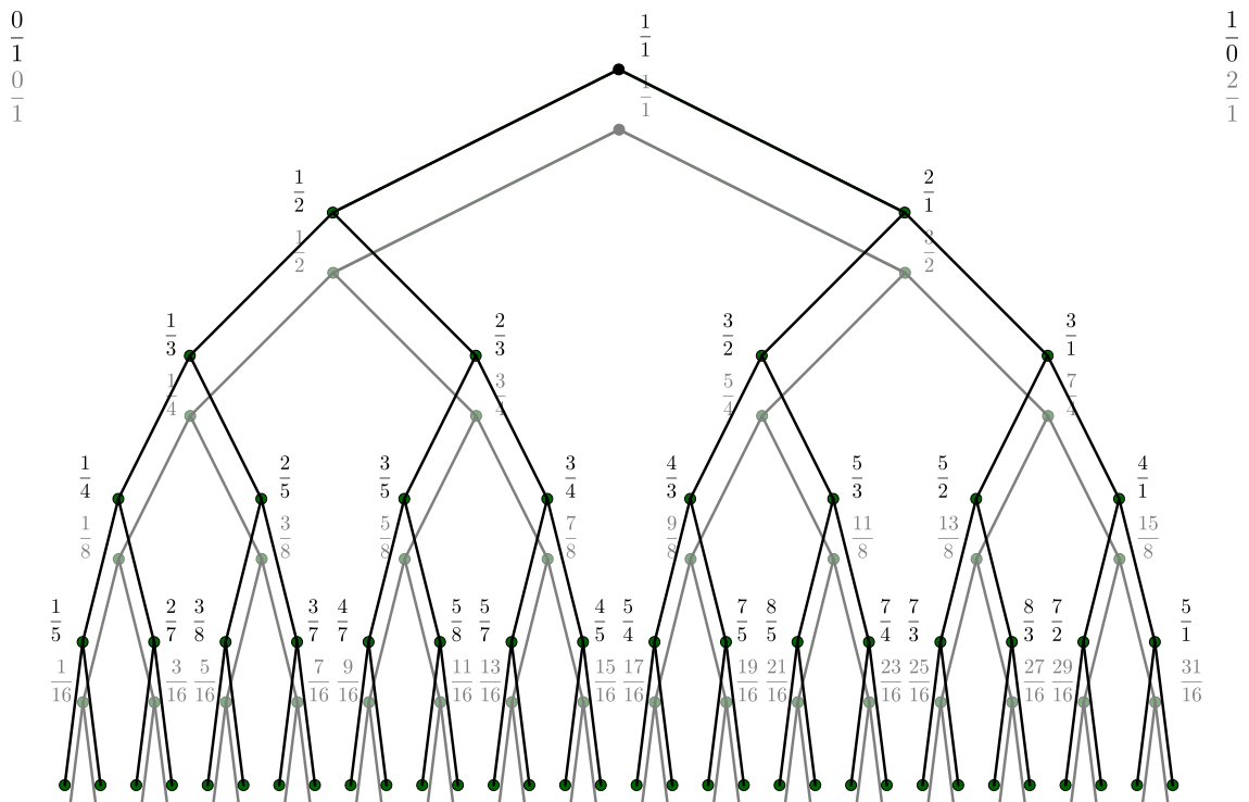
Tree of Fractions

There’s an entirely separate structure which contains all rationals in least terms. It relies on an operation between two fractions called the mediant. For two rational numbers in least terms p and q, such that p < q, the mediant is designated p ⊕ q and will:

1. also be in least terms (with some exceptions, see below),
2. be larger than p, and
3. be smaller than q

\begin{gather*} p = {a \over b} < {c \over d} = q, \quad \gcd(a,b) = \gcd(c,d) = 1 \\ \\ p < p \oplus q < q \quad \phantom{\gcd(a+c, b+d) = 1} \\ \\ {a \over b} < {a+c \over b+d} < {c \over d}, \quad \gcd(a+c, b+d) = 1 \end{gather*}

We know our sequence of rationals starts with 1/1, 1/2, and 2/1. If we start as before with 1/1 and want to get the other quantities, then we can take its mediants with 0/1 and 1/0, respectively (handwaving the fact that the latter isn’t a legitimate fraction).

\begin{align*} && && \large{1 \over 1} && && \\ { \oplus {0 \over 1} } && \large{/} && && \large{\backslash} ~ && \oplus {1 \over 0} \\ && \large{1 \over 2} && && \large{2 \over 1} && \end{align*}

We might try continuing this pattern by doing the same thing to 1/2. We can take its mediant with 0/1 to get 1/3. Unfortunately, the mediant of 1/2 and 1/0 is 2/2 (as is the mediant of 2/1 with 0/1), which isn’t in least terms, and has already appeared as 1/1.

We could try another fraction that’s appeared in the tree. Unfortunately, 2/1 suffers from the same issue as 1/0 – 1/2 ⊕ 2/1 = 3/3, which is the same quantity as before, despite both fractions being in least terms. On the other hand, 1/2 ⊕ 1/1 = 2/3, which is in least terms. Similarly, 2/1 ⊕ 1/1 is 3/2, its reciprocal.

\begin{align*} && && \large{1 \over 2} && && \\ { \oplus {0 \over 1} } && \large{/} && && \large{\backslash} ~ && \oplus {1 \over 1} \\ && \large{1 \over 3} && && \large{2 \over 3} && \end{align*} \qquad \qquad \begin{align*} && && \large{2 \over 1} && && \\ { \oplus {1 \over 1} } && \large{/} && && \large{\backslash} ~ && \oplus {1 \over 0} \\ && \large{3 \over 2} && && \large{3 \over 1} && \end{align*}

The trick is to notice that a step to the left “updates” what the next step to the right looks like. Steps to the right behave symmetrically. For example, in the row we just generated, the left child of 2/3 is its mediant with 1/2, its right child is its mediant with 1/1.

Continuing this iteration ad infinitum forms the Stern-Brocot tree. A notable feature of this is that it is a binary search tree (of infinite height). This means that for any node, the value at the node is greater than all values in the left subtree and less than all values in the right subtree.

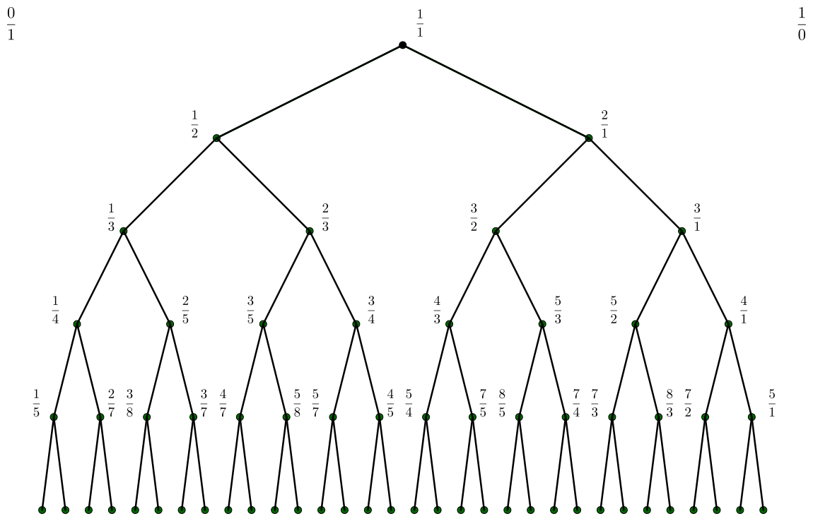
There’s a bit of a lie in presenting the tree like this. As a binary tree, it’s most convenient to show the nodes spaced evenly, but the distance between 1/1 and 2/1 is not typically seen as the same as the distance between 1/1 and 1/2.

We can implement this in Haskell using Data.Tree. This package actually lets you describe trees with any number of child nodes, but we only need two for the sake of the Stern-Brocot tree.

import Data.Tree

-- Make a tree by applying the function `make` to each node
-- Start with the root value (1, 1), along with
-- its left and right steps, (0, 1) and (1, 0)
sternBrocot = unfoldTree make ((1,1), (0,1), (1,0)) where
  -- Place the first value in the tree, then describe the next
  -- values for `make` in a list:
  make (v@(vn, vd), l@(ln, ld), r@(rn, rd))
    = (v, [
      -- the left value, and its left (unchanged) and right steps...
      ((ln + vn, ld + vd), l, v),
      -- and the right value, and its left and right (unchanged) steps
      ((vn + rn, vd + rd), v, r)
    ])

Cutting the Tree Down

We’re halfway there. All that remains is to read off every value in the tree as a sequence. Perhaps the most naive way would be to read off by always following the left or right child. Unfortunately, these give some fairly dull sequences.

treePath :: [Int] -> Tree a -> [a]
treePath xs (Node y ys)
    -- If we don't have any directions (xs), or the node
    -- has no children (ys), then there's nowhere to go
  | null xs || null ys = [y]
    -- Otherwise, go down subtree "x", then recurse with that tree
    -- and the rest of the directions (xs)
  | otherwise = y:treePath (tail xs) (ys !! head xs)

-- Always go left (child 0)
-- i.e., numbers with numerator 1
mapM_ print $ take 10 $ treePath (repeat 0) sternBrocot

-- Always go right (child 1)
-- i.e., numbers with denominator 1
mapM_ print $ take 10 $ treePath (repeat 1) sternBrocot

(1,1)
(1,2)
(1,3)
(1,4)
(1,5)
(1,6)
(1,7)
(1,8)
(1,9)
(1,10)

(1,1)
(2,1)
(3,1)
(4,1)
(5,1)
(6,1)
(7,1)
(8,1)
(9,1)
(10,1)

Rather than by following paths in the tree, we can instead do a breadth-first search. In other words, we read off each row individually, in order. This gives us our sequence of rational numbers with no repeats.

\begin{gather*} \begin{align*} \mathbb{N^+}& ~\rightarrow~ \mathbb{Q} \\ n & ~\mapsto~ \text{bfs}[n] \end{align*} \\ \\ 1 \mapsto 1/1,~ \\ 2 \mapsto 1/2,\quad 3 \mapsto 2/1,~ \\ 4 \mapsto 1/3,\quad 5 \mapsto 2/3, \quad 6 \mapsto 3/2, \quad 7 \mapsto 3/1,~ ... \end{gather*}

For convenience, this enumeration is given starting from 1 rather than from 0. This numbering makes it clearer that each row starts with a power of 2, since the structure is a binary tree, and the complexity doubles with each row. The enumeration could just as easily start from 0 by starting with \N, then getting to \N^+ with n \mapsto n+1.

We can also write a breadth-first search in Haskell, for posterity:

bfs :: Tree a -> [a]
bfs (Node root children) = bfs' root children where
  -- Place the current node in the list
  bfs' v []               = [v]
  -- Pluck one node off our list of trees, then recurse with
  -- the rest, along with that node's children
  bfs' v ((Node y ys):xs) = v:bfs' y (xs ++ ys)

sternBrocotRationals = bfs sternBrocot

mapM_ putStrLn $ take 10 $ map showAsRational sternBrocotRationals

(1,1) = 1/1
(1,2) = 1/2
(2,1) = 2/1
(1,3) = 1/3
(2,3) = 2/3
(3,2) = 3/2
(3,1) = 3/1
(1,4) = 1/4
(2,5) = 2/5
(3,5) = 3/5

The entries in this enumeration have already been given.

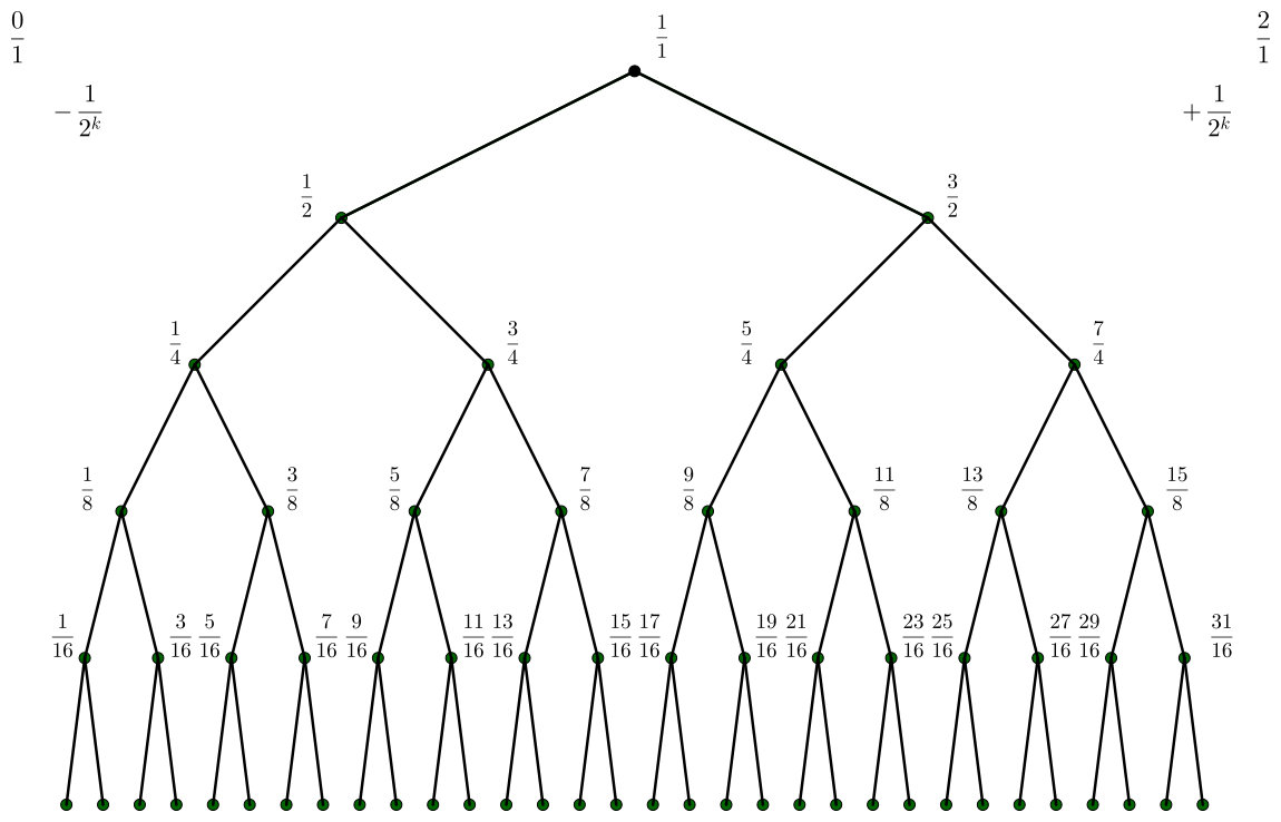
Another Tree

Another tree of fractions to consider is the tree of binary fractions. These fractions simply consist of odd numbers divided by powers of two. The most convenient way to organize these into a tree is to keep denominators equal if the nodes have the same depth from the root. We also stipulate that we arrange the nodes as a binary search tree, like the Stern-Brocot tree.

The tree starts from 1/1 as before. Its children have denominator 2, so we have 1/2 to the left and 3/2 to the right. This is equivalent to subtracting 1/2 for the left step and adding 1/2 for the right step. At the next layer, we want fractions with denominator 1/4, and do similarly. In terms of adding and subtracting, we just use 1/4 instead of 1/2.

We can describe this easily in Haskell:

-- Start with 1/1 (i.e., (1, 1))
binFracTree = unfoldTree make (1,1) where
  -- Place the first value in the tree, then describe the next
  -- values for `make` in a list:
  make v@(vn, vd)
    = (v, [
      -- double the numerator and denominator, then subtract 1 from the numerator
      (2*vn - 1, 2*vd),
      -- same, but add 1 to the numerator instead
      (2*vn + 1, 2*vd)
    ])

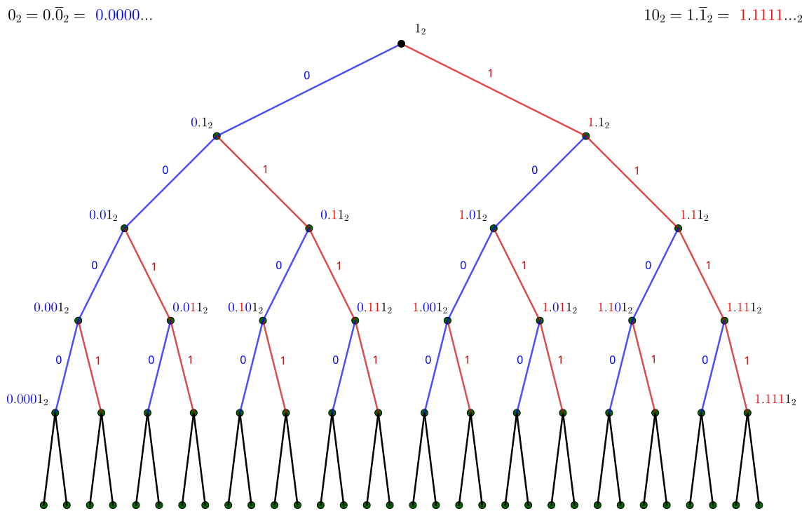
The entries of this tree have an additional interpretation when converted to their binary expansions. These fractions always terminate in a “1” in binary, but ignoring this final entry, starting from the root and following “left” for 0 and “right” for 1 places us at that fraction in the tree. In other words, the binary expansions encode the path from the root to the node.

Why Bother?

The tree of binary fractions and the Stern-Brocot tree are both infinite binary search trees, so we might imagine overlaying one tree over the other, pairing up the individual entries.

In Haskell, we can pair up entries recursively:

zipTree :: Tree a -> Tree b -> Tree (a,b)
-- Pair the values in the nodes together, then recurse with the child trees
zipTree (Node x xs) (Node y ys) = Node (x,y) $ zipWith zipTree xs ys

binarySBTree = zipTree sternBrocot binFracTree

Conveniently, both left subtrees of the root fall in the interval (0, 1). It also pairs up 1 and 1/2 with themselves. Doing so establishes a bijection between the rationals and the binary rationals in that interval. Rationals are more continuous than integers, so it might be of some curiosity to plot this function. We only have to look at a square over the unit interval. Doing so reveals a curious shape:

import Data.Tuple (swap)
import Data.List (sort)
import Data.Bifunctor (bimap, first)

leftSubtree (Node _ (x:_)) = x

-- Divide entries of the (zipped) trees
(</>) (a,b) = fromIntegral a / fromIntegral b :: Double
binarySBDoubles n = take n $ map (bimap (</>) (</>)) $ bfs $ leftSubtree binarySBTree

(MPL.tightLayout <>) $ uncurry MPL.plot $ unzip $ sort $ map swap $ binarySBDoubles 250
(MPL.tightLayout <>) $ uncurry MPL.plot $ unzip $ sort $ binarySBDoubles 250

Binary rationals on the x-axis, rationals on the y-axis

Rationals on the x-axis, binary rationals on the y-axis

The plot on the right which maps the rationals to the binary rationals is known as Minkowski’s question mark function. Notice that this function is nearly 1/2 for values near 1/2 (nearly 1/4 for values near 1/3, nearly 1/8 for values near 1/4, etc.).

I’m Repeating Myself

The inverse question mark map (which I’ll call ¿ for short), besides mapping binary rationals to rationals, has an interesting relationship with other rational numbers. Recall that we only defined the function in terms of fractions which happen to have finite binary expansions. Those with infinite binary expansions, such as 1/3 (and indeed, any fraction whose denominator isn’t a power of 2) aren’t defined.

\begin{gather*} {1 \over 2} = 0.1_2 \\ {1 \over 3} = 0.\overline{01} = 0.\textcolor{red}{01}\textcolor{green}{01}\textcolor{blue}{01}... \\ {1 \over 4} = 0.01_2 \\ {1 \over 5} = 0.\overline{0011} = 0.\textcolor{red}{0011}\textcolor{green}{0011}\textcolor{blue}{0011}... \\ \vdots \end{gather*}

We can persevere if we continue to interpret the binary strings as a path in the tree. This means that for 1/3, we go left initially, then alternate between going left and right. As we do so, let’s take note of the values we pass along the way:

-- Follow the path described by the binary expansion of 1/3
oneThirdPath = treePath (0:cycle [0,1]) $ zipTree sternBrocot binFracTree

trimTo n x = if length x > n then "(too big to show)" else x

treePathColumns = columns (\(_, f) v -> f v) (\(l, _) -> Headed l) [
    (stringCell "n",
      stringCell . fromEither . fmap show),
    (stringCell "Binary fraction",
      stringCell . fromEither . fmap (trimTo 10 . showAsRational' . snd . (oneThirdPath !!))),
    (stringCell "Binary fraction (decimal)",
      stringCell . fromEither . fmap (show . (</>) . snd . (oneThirdPath !!))),
    (stringCell "Stern-Brocot rational",
      stringCell . fromEither . fmap (trimTo 10 . showAsRational' . fst . (oneThirdPath !!))),
    (stringCell "Stern-Brocot rational (decimal)",
      stringCell . fromEither . fmap (show . (</>) . fst . (oneThirdPath !!)))
  ] where
  fromEither = either id id

renderTable treePathColumns (map Right [0..8] ++ [Left "...", Right 100, Left "..."])

n	Binary fraction	Binary fraction (decimal)	Stern-Brocot rational	Stern-Brocot rational (decimal)
0	1/1	1.0	1/1	1.0
1	1/2	0.5	1/2	0.5
2	1/4	0.25	1/3	0.3333333333333333
3	3/8	0.375	2/5	0.4
4	5/16	0.3125	3/8	0.375
5	11/32	0.34375	5/13	0.38461538461538464
6	21/64	0.328125	8/21	0.38095238095238093
7	43/128	0.3359375	13/34	0.38235294117647056
8	85/256	0.33203125	21/55	0.38181818181818183
...	...	...	...	...
100	(too big to show)	0.3333333333333333	(too big to show)	0.3819660112501052
...	...	...	...	...

convergentsOneThird = map ((</>) . snd) oneThirdPath
convergentsSBNumber = map ((</>) . fst) oneThirdPath

plotSequence n = uncurry MPL.plot . unzip . take n . zip ([0..] :: [Int])

(MPL.tightLayout <>) $ plotSequence 20 convergentsOneThird
(MPL.tightLayout <>) $ plotSequence 20 convergentsSBNumber

Binary convergents of 1/3

¿ applied to binary convergents of 1/3, which also appear to converge

Both sequences appear to converge to a number, with the binary fractions obviously converging to 1/3. The rationals from the Stern-Brocot don’t appear to be converging to a repeating decimal. Looking closer, the numerators and denominators of the fractions appear to come from the Fibonacci numbers. In fact, the quantity that the fractions approach is 2 - \varphi, where φ is the golden ratio. This number is the root of the polynomial x^2 - 3x + 1.

In fact, all degree 2 polynomials have roots that are encoded by a repeating path in the Stern-Brocot tree. Put another way, ¿ can be extended to map rationals other than binary fractions to quadratic roots (and ? maps quadratic roots to rational numbers). This is easier to understand when writing the quantity as its continued fraction expansion, but that’s an entirely separate discussion.

Either way, it tells us something interesting: not only can all rational numbers be enumerated, but so can quadratic irrationals.

The Other Side

I’d like to briefly digress from talking about enumerations and mention the right subtree. The question mark function, as defined here, is only defined on numbers between 0 and 1 (and even then, technically only rational numbers). According to Wikipedia’s definition, the question mark function is quasi-periodic – ?(x + 1) = ?(x) + 1. On the other hand, according to the definition by pairing up the two trees, rationals greater than 1 get mapped to binary fractions between 1 and 2.

binarySBDoublesAll n = take n $ map (bimap (</>) (</>)) $ bfs binarySBTree

(MPL.tightLayout <>) $ uncurry MPL.plot $
  unzip $ sort $ binarySBDoublesAll 250
(MPL.tightLayout <>) $ uncurry MPL.plot $
  unzip $ map (first log) $ sort $ binarySBDoublesAll 250

(a) linear x-axis

(b) (base 2)-logarithmic x-axis

Question mark function including right subtree

Here are graphs describing our question mark function, on linear and logarithmic plots. Instead of repeating, the function continues its self-similar behavior as it proceeds onward to infinity (logarithmically). The right graph stretches from -∞, where its value would be 0, to ∞, where its value would be 2.

Personally, I like this definition a bit better, if only because it matches other ways of thinking about the interval (0, 1). For example,

• In topology, it’s common to show that this interval is homeomorphic to the entire real line
• It’s similar to the rational functions which appear in stereography, which continue to infinity instead of being periodic
• It showcases how the Stern-Brocot tree sorts rational numbers by complexity better

However, it’s also true that different definitions are good for different things. For example, periodicity matches the intuition that numbers can be decomposed into a fractional and integral part. Integral parts grow without bound, while fractional parts are periodic, just like the function would be.

Closing

I’d like to draw this discussion of enumerating numbers to a close for now. I wrote this article to establish some preliminaries regarding another post that I have planned. On the other hand, since I was describing the Stern-Brocot tree, I felt it also pertinent to show the question mark function, since it’s a very interesting self-similar curve. Even then, I have shown them as a curiosity instead of giving them their time in the spotlight.

I have omitted some things I would like to have discussed, such as order type, and enumerating things beyond just the quadratic irrationals. I may return to some of these topics in the future, such as to show a way to order integer polynomials.

Diagrams created with GeoGebra (because trying to render them in LaTeX would have taken too long) and Matplotlib.

Footnotes

1. That is, if you cover your eyes and pretend that undefined will never happen, and if you ignore that Int is bounded, unlike Integer.