Expressing rotation mathematically can be rather challenging, even in two dimensional space. Typically, the subject is approached from complicated-looking rotation matrices, with the occasional accompanying comment about complex numbers. The challenge only increases when examining three dimensional space, where everyone has different ideas about the best implementations. In what follows, I attempt to provide a derivation of 2D and 3D rotations based in intuition and without the use of trigonometry.
Complex Numbers: 2D Rotations
As points in the plane, multiplication between complex numbers is frequently analyzed as a combination of scaling (a ratio of two scales) and rotation (a point on the complex unit circle). However, the machinery used in these analyses usually expresses complex numbers in a polar form involving the complex exponential. This leverages prior knowledge of trigonometry and some calculus, and in fact obfuscates the algebraic properties of complex numbers. Neither concept is truly necessary to understand points on the complex unit circle, or complex number multiplication in general.
A review of complex multiplication
A complex number z = a + bi multiplies with another complex number w = c + di in the obvious way: by distributing over addition.
zw = (a + bi)(c + di) = ac + bci + adi + bdi^2 = (ac - bd) + i(ad + bc)
z also has associated to it a conjugate z^* = a - bi. The product zz^* is the norm a^2 + b^2, a positive real quantity whose square root is typically called the magnitude of the complex number. Taking the square root is frequently unnecessary, as many of the properties of this quantity do not depend on this normalization.
One such property is that for two complex numbers z and w, the norm of the product is the product of the norm.
\begin{align*}
(zw)(zw)^* &= (ac - bd)^2 + (ad + bc)^2
\\
&= a^2c^2 - 2abcd + b^2d^2 + a^2d^2 + 2abcd + b^2c^2
\\
&= a^2c^2 + b^2d^2 + a^2d^2 + b^2c^2
= a^2(c^2 + d^2) + b^2(c^2 + d^2)
\\
&= (a^2 + b^2)(c^2 + d^2)
\end{align*}
Conjugation also distributes over multiplication, and complex numbers possess multiplicative inverses. Also, the norm of the multiplicative inverse is the inverse of the norm.
\begin{gather*}
z^*w^* = (a - bi)(c - di) = ac - bci - adi + bdi^2
\\
= (ac - bd) - i(ad + bc) = (zw)^{*}
\\
{1 \over z} = {z^{*} \over z z^{*}} = {a - bi \over a^2 + b^2}
\\[14pt]
\left({1 \over z}\right)
\left({1 \over z}\right)^{*}
= {1 \over zz^{*}} = {1 \over a^2 + b^2}
\end{gather*}
A final interesting note about complex multiplication is the product z^{*} w
z^{*} w = (a - bi)(c + di) = ac - bci + adi - bdi^2 = (ac + bd) + i(ad - bc)
The real part is the same as the dot product (a, c) \cdot (b, d) and the imaginary part looks like the determinant of \begin{pmatrix}a & b \\ c & d\end{pmatrix}. This shows the inherent value of complex arithmetic, as both of these quantities have important interpretations in vector algebra.
Onto the Circle
If zz^{*} = a^2 + b^2 = 1, then z lies on the complex unit circle. Since the norm is 1, a general complex number w has the same norm as its product with z, zw. Specifically, if w is 1, multiplication by z can be seen as the rotation that maps 1 to z. But how do you describe a point on the unit circle?
Simple. For any complex w, there are three other complex numbers that are guaranteed to share its norm: -w, w^{*}, and -w^{*}. Dividing any one of these numbers by another results in a complex number on the unit circle. Dividing w by -w is boring, since that just results in -1. However, division by w^* turns out to be important:
\begin{align*}
z &= {w \over w^*} =
\left( {c + di \over c - di} \right)
\left( {c + di \over c + di} \right) = 1
\\[8pt]
&= {(c^2 - d^2) + (2cd)i \over c^2 + d^2}
\end{align*}
Dividing the numerator and denominator of this expression through by c^2 yields an expression in t = d/c, where t can be interpreted as the slope of the line joining 0 and w. Slopes range from -\infty to \infty, which means that the variable t does as well.
\begin{align*}
{(c^2 - d^2) + (2cd)i \over c^2 + d^2}
&= {1/c^2 \over 1/c^2} \cdot {(c^2 - d^2) + (2cd)i \over c^2 + d^2}
\\
&= {(1 - d^2/c^2) + (2d/c)i \over 1 + d^2/c^2}
= {(1 - t^2) + (2t)i \over 1 + t^2}
\\
&= {1 - t^2 \over 1 + t^2} + i{2t \over 1 + t^2} = z(t)
\end{align*}
This gives us a point z on the unit circle. Its reciprocal is:
{1 \over z} = {z^{*} \over zz^{*}} = z^{*}
Applying the same operation to z as we did to w gives us z / z^{*} = z^2, or as an action on points, the rotation from 1 to z^2.
This demonstrates the decomposition of the rotation into two parts. For a general complex number w which may not lie on the unit circle, multiplication by this number dilates the complex plane as well rotating 1 toward the direction of w. Then, division by w^{*} undoes the dilation and performs the rotation again. General (i.e., non-unit) rotations must occur in pairs.
Two Halves, Twice Over
Plugging in -1, 0, and 1 for t reveals some interesting behavior: z(0) = 1 + 0i, z(1) = 0 + 1i, and z(-1) = 0 - 1i. Assuming continuity, this shows that t \in (-1, 1) plots the semicircle in the right half-plane. The other half of the circle comes from t with magnitude greater than 1, and the point where z(t) = -1 exists if we admit the extra point t = \pm \infty.
Is it possible to get the other half into a nicer interval? No problem, just double the rotation.
\begin{align*}
z(t)^2 &= (\Re[z]^2 - \Im[z]^2) + i(2\Re[z]\Im[z])
\\[8pt]
&= {(1 - t^2)^2 - (2t)^2 \over (1 + t^2)^2} + i{2(1 - t^2)(2t) \over (1 + t^2)^2}
\\[8pt]
&= {1 - 6t^2 + t^4 \over 1 + 2t^2 + t^4}
+ i {4t - 4t^3 \over 1 + 2t^2 + t^4}
\end{align*}
Now z(-1)^2 = z(1)^2 = -1 and the entire circle fits in the interval [-1, 1]. This action of squaring z means that as t ranges from -\infty to \infty, the point z^2 loops around the circle twice, since the unit rotation z is applied twice.
Plotting Transcendence
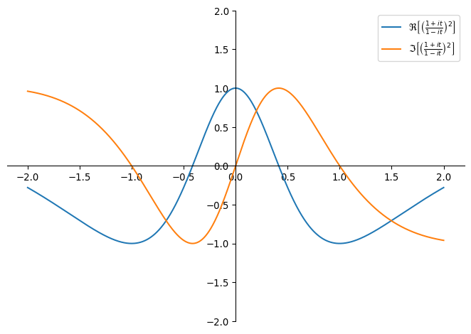
Let’s go on a brief tangent and compare these expressions to their transcendental trigonometric counterparts. Graphing the real and imaginary parts separately shows how much they resemble \cos(\pi t) and \sin(\pi t) around zero.
Ideally, the zeroes of the real part should occur at t = \pm 1/2, since \cos(\pm \pi/2) = 0. Instead, they occur at
\begin{align*}
0 &= 1 - 6t^2 + t^4
= (t^2 - 2t - 1)(t^2 + 2t - 1)
\\
&\implies t = \pm {1 \over \delta_s} = \pm(\sqrt 2 - 1) \approx \pm 0.414
\end{align*}
With a bit of polynomial interpolation, this can be rectified. A cubic interpolation between the expected and actual values is given by:
\begin{gather*}
P(x) = ax^3 + bx^2 + cx + d
\\
\begin{pmatrix}
1 & 0 & 0 & 0 \\
1 & 1/2 & 1/4 & 1/8 \\
1 & -1/2 & 1/4 & -1/8 \\
1 & 1 & 1 & 1
\end{pmatrix} \begin{pmatrix}
d \\
c \\
b \\
a
\end{pmatrix} = \begin{pmatrix}
0 \\
\sqrt 2 - 1 \\
-\sqrt 2 + 1 \\
1
\end{pmatrix}
\\
\implies \begin{pmatrix}
d \\
c \\
b \\
a
\end{pmatrix} = \begin{pmatrix}
0 \\
-3 + 8\sqrt 2/3 \\
0 \\
4 - 8\sqrt 2/3
\end{pmatrix}
\implies P(x) \approx 0.229 x^3 + 0.771x
\end{gather*}
The error over the interval [-1, 1] in these approximations is around 1% (RMS).
Notably, this interpolating polynomial is entirely odd, which gives it some symmetry about 0. Along with being a very good approximation, it has the feature that a rotation by an nth of a turn is about z(P(1/n))^2. The approximation be improved further by taking z to higher powers and deriving a higher-order interpolating polynomial.
It is impossible to shrink this error to 0 because the derivative of the imaginary part at t = 1 would be π. But the imaginary part is a rational expression, so its derivative is also a rational expression. Since π is transcendental, there must always be some error.
Even though it is arguably easier to calculate, there probably isn’t a definite benefit to this approximation. For example,
- Other accurate approximants for sine and cosine can be calculated directly from their power series.
- There are no inverse functions like
acos or asin to complement these approximations.
- This isn’t that bad, since I have refrained from describing rotations with an angle (i.e., the quantity returned by these functions). Even so, the inverse functions have their use cases.
- Trigonometric functions can be hardware-accelerated (at least in some FPUs).
- If no such hardware exists, approximations of
sin and cos can be calculated by software beforehand and stored in a lookup table (which is also probably involved at some stage of the FPU).
Elaborating on the latter two points, using a lookup table means evaluation happens in roughly constant time. A best-case analysis of the above approximation, given some value t is…
| p = t \cdot (0.228763834 \cdot t \cdot t + 0.771236166) |
1 |
3 |
|
| q = p \cdot p |
|
1 |
|
| r = 1 + q |
1 |
|
|
| c = { 1 - q \over r} |
1 |
|
1 |
| s = { p + p \over r} |
1 |
|
1 |
| real = c \cdot c - s \cdot s |
1 |
2 |
|
| imag = c \cdot s + c \cdot s |
1 |
1 |
|
| Total |
6 |
7 |
2 |
…or 15 FLOPs.
On a more optimistic note, a Monte Carlo test of the above approximation on my computer yields promising results when compared with GCC’s libm implementations of sin, cos, and cexp.
Timing for 10000000 math.h sin and cos: 2838358ns
Timing for 10000000 approximations: 1239784ns
Approximation faster, speedup: 1598574ns (2.29x)
Squared error in cosines (100000 runs):
    Average: 0.000051 (0.713743% error)
    Largest: 0.000174 (1.320551% error)
        Input:       0.729202
        Value:       -0.659428
        Approximation:   -0.672634
Squared error in sines (100000 runs):
    Average: 0.000070 (0.835334% error)
    Largest: 0.000288 (1.698413% error)
        Input:       0.842206
        Value:       0.475669
        Approximation:   0.458685
Timing for 10000000 complex.h cexp:   4725615ns
Timing for 10000000 approximations: 1780325ns
Approximation faster, speedup: 2945290ns (2.65x)
Squared error in cosines (100000 runs):
    Average: 0.000051 (0.713743% error)
    Largest: 0.000174 (1.320551% error)
        Input:       0.729202
        Value:       -0.659428
        Approximation:   -0.672634
Squared error in sines (100000 runs):
    Average: 0.000070 (0.835334% error)
    Largest: 0.000288 (1.698413% error)
        Input:       0.842206
        Value:       0.475669
        Approximation:   0.458685
For the source which I used to generate this output, see the repository linked at the bottom of this article.
Even though results can be inaccurate, this exercise in the algebraic manipulation of complex numbers is fairly interesting since it requires no calculus to define, unlike sine, cosine, and their Padé approximants (and to a degree, π).
From Circles to Spheres
The expression for complex points on the unit circle coincides with the stereographic projection of a circle. This method is achieved by selecting a point on the circle, fixing t along a line (such as the y-axis), and letting t range over all possible values.
The equations of the line and circle appear in the diagram above. Through much algebra, expressions for x and y as functions of t can be formed.
\begin{align*}
y &= t(x + 1)
\\
1 &= x^2 + y^2 = x^2 + (tx + t)^2
\\
&= x^2 + t^2x^2 + 2t^2 x + t^2
\\[14pt]
{1 \over t^2 + 1} -\ {t^2 \over t^2 + 1}
&= x^2 + {t^2 \over t^2 + 1} 2x
\\
{1 -\ t^2 \over t^2 + 1} + \left( {t^2 \over t^2 + 1} \right)^2
&= \left(x + {t^2 \over t^2 + 1} \right)^2 + {t^2 \over t^2 + 1}
\\
{1 -\ t^4 \over (t^2 + 1)^2} + {t^4 \over (t^2 + 1)^2}
&= \left(x + {t^2 \over t^2 + 1} \right)^2
\\
{1 \over (t^2 + 1)^2}
&= \left(x + {t^2 \over t^2 + 1} \right)^2
\\
{1 \over t^2 + 1}
&= x + {t^2 \over t^2 + 1}
\\
x &= {1 -\ t^2 \over 1 + t^2}
\\
y &= t(x + 1)
= t\left( {1 -\ t^2 \over 1 + t^2} + {1 + t^2 \over 1 + t^2} \right)
\\
&= {2t \over 1 + t^2}
\end{align*}
These are exactly the same expressions which appear in the real and imaginary components of the ratio between 1 + ti and its conjugate.
Compared to the algebra using complex numbers, this is quite a bit more work. One might ask whether, given a proper arithmetic setting, this can be extended to three dimensions. In other words, we want to find the projection of a sphere using some new number system analogously to the circle with respect to complex numbers.
Algebraic Projection
The simplest thing to do is try it out. Let’s say an extended number h = 1 + si + tj has a conjugate of h^{*} = 1 - si - tj. Then, following our noses:
\begin{gather*}
{h \over h^{*}} = {1 + si + tj \over 1 - si - tj}
= \left({1 + si + tj \over 1 - si - tj}\right)
\left({1 + si + tj \over 1 + si + tj}\right)
\\[8pt]
= {
1 + si + tj + si + s^2i^2 + stij + tj + stji + t^2j^2
\over 1 - si - tj + si - s^2 i^2 - stij + tj - stji - t^2j^2
}
\end{gather*}
While there is some cancellation in the denominator, both products are rather messy. To get more cancellation, we can add some nice algebraic properties between i and j. If we let i and j be anticommutative (meaning that ij = -ji) then stij cancels with stji. So that the denominator is totally real (and therefore can be guaranteed to divide), we can also assert that i^2 and j^2 are both real. Then the expression becomes
{1 + si + tj \over 1 - si - tj}
= {1 + s^2i^2 + t^2j^2 \over 1 - s^2 i^2 - t^2 j^2}
+ i{2s \over 1 - s^2 i^2 - t^2 j^2}
+ j{2t \over 1 - s^2 i^2 - t^2 j^2}
If it is chosen that i^2 = j^2 = -1, this produces the correct equations parametrizing the unit sphere (see Wikipedia).
{h \over h^{*}} = {1 - s^2 - t^2 \over 1 + s^2 + t^2}
+ i{2s \over 1 + s^2 + t^2}
+ j{2t \over 1 + s^2 + t^2}
One can also check that this makes the squares of the real, i, and j components sum to 1.
If both i and j anticommute, then their product also anticommutes with both i and j.
\textcolor{red}{ij}j = -j\textcolor{red}{ij}
~,~ i\textcolor{red}{ij} = -\textcolor{red}{ij}i
Calling this product k and noticing that k^2 = (ij)(ij) = -ijji = i^2 = -1 completely characterizes the quaternions.
Other projections
Choosing different values for i^2 and j^2 yield different shapes than a sphere. If you know a little group theory, you might know there are only two nonabelian (noncommutative) groups of order 8:
In the latter group, j and k are both imaginary, but square to 1 (i still squares to -1).
Changing the sign of one (or both) of the imaginary squares in the expression h / h^{*} above switches the multiplicative structure from quaternions to the dihedral group. In this group, picking i^2 = -j^2 = -1 parametrizes a hyperboloid of one sheet, and picking i^2 = j^2 = 1 parametrizes a hyperboloid of two sheets.
Quaternions and Rotation
We’ve already established that complex numbers are useful for describing 2D rotations. They also elegantly describe the stereographic projection of a circle. Consequently, since quaternions elegantly describe the stereographic projection of a sphere, they are useful for 3D rotations.
Since the imaginary units i, j, and k are anticommutative, a general quaternion does not commute with other quaternions like complex numbers do. This embodies a difficulty with 3D rotations in general: unlike 2D rotations, they do not commute.
Only three of the four components in a quaternion are necessary to describe a point in 2D space. The ijk subspace is ideal since the three imaginary axes are symmetric (i.e., they all square to -1). Quaternions in this subspace are called vectors. Another reason for using the ijk subspace comes from considering a point u = ai + bj + ck on the unit sphere (a^2 + b^2 + c^2 = 1). Then the square of this point is:
\begin{align*}
u^2 &= (ai + bj + ck)(ai + bj + ck)
\\
&= a^2i^2 + abij + acik + abji + b^2j^2 + bcjk + acki + bckj + c^2k^2
\\
&= (a^2 + b^2 + c^2)(-1) + ab(ij + ji) + ac(ik + ki) + bc(jk + kj)
\\
&= -1 + 0 + 0 + 0
\end{align*}
This property means that u behaves similarly to a typical imaginary unit. If we form pseudo-complex numbers of the form a + b u, then {1 + tu \over 1 - tu} = \alpha + \beta u specifies some kind of rotation in terms of the parameter t. As with complex numbers, the inverse rotation is the conjugate 1 - tu \over 1 + tu.
Another useful feature of quaternion algebra involves symmetry transformations of the imaginary units. If an imaginary unit (one of i, j, k) is left-multiplied by a quaternion q and right-multiplied by its conjugate q^{*}, then the result is still imaginary. In other words, if p is a vector, then qpq^{*} is also a vector since i, j, and k form a basis and multiplication distributes over addition. I will not demonstrate this fact, as it requires a large amount of algebra.
These two features combine to characterize a transformation for a vector quaternion. For a vector p, if q_u(t) is a “rotation” as above for a point u on the unit sphere, then another vector (the image of p) can be described by
\begin{gather*}
qpq^* = qpq^{-1}
= \left({1 + tu \over 1 - tu}\right) p \left({1 - tu \over 1 + tu}\right)
= (\alpha + \beta u)p(\alpha - \beta u)
\\[4pt]
= (\alpha + \beta u)(\alpha p - \beta pu)
= \alpha^2 p - \alpha \beta pu + \alpha \beta up - \beta^2 upu
\end{gather*}
Testing a Transformation
3D space contains 2D subspaces. If this transformation is a rotation, then a 2D subspace will be affected in a way which can be described more simply by complex numbers. For example, if u = k and p = xi + yj, then this can be expanded as:
\begin{align*}
qpq^{-1} &= (\alpha + \beta k)(xi + yj)(\alpha - \beta k)
\\[10pt]
&= \alpha^2(xi + yj) - \alpha \beta (xi + yj)k + \alpha \beta k(xi + yj) - \beta^2 k(xi + yj)k
\vphantom{\over}
\\[10pt]
&= \alpha^2(xi + yj) - \alpha \beta(-xj + yi) + \alpha \beta(xj - yi) - \beta^2(xi + yj)
\\[10pt]
&= (\alpha^2 - \beta^2)(xi + yj) + 2\alpha \beta(xj - yi)
\\[10pt]
&= [(\alpha^2 - \beta^2)x - 2\alpha \beta y]i + [(\alpha^2 - \beta^2)y + 2\alpha \beta x]j
\end{align*}
If p is rewritten as a vector (in the linear algebra sense), then this final expression can be rewritten as a linear transformation of p:
\begin{align*}
\begin{pmatrix}
(\alpha^2 - \beta^2)x - 2 \alpha \beta y \\
(\alpha^2 - \beta^2)y + 2 \alpha \beta x
\end{pmatrix}
&= \begin{pmatrix}
\alpha^2 - \beta^2 & -2\alpha \beta \\
2\alpha \beta & \alpha^2 - \beta^2
\end{pmatrix}
\begin{pmatrix}
x \\
y
\end{pmatrix}
\\
&= \begin{pmatrix}
\alpha & -\beta \\
\beta & \alpha
\end{pmatrix}^2
\begin{pmatrix}
x \\
y
\end{pmatrix}
\end{align*}
The complex number \alpha + \beta i is isomorphic to the matrix on the second line. Since \alpha and \beta were chosen so to lie on “a” complex unit circle, this means that the vector (x, y) is rotated by \alpha + \beta i twice. This also demonstrates that u specifies the axis of rotation, or equivalently, the plane of a great circle. This means that the “some kind of rotation” specified by q is a rotation around the great circle normal to u.
The double rotation resembles the half-steps in the complex numbers, where 1 + ti performs a dilation, {1 \over 1 - ti} reverses it, and together they describe a rotation. The form qpq^{-1} is similar to this – the q on the left performs some transformation which is (partially) undone by the q^{-1} on the right. In this case, since q’s conjugate is its inverse and quaternions do not commute, the only thing to do without the transformation being trivial is to sandwich p between them.
As shown above, the product of a vector with itself should be totally real and equal to the negative of the norm of p, the sum of the squares of its components. The rotated p shares the same norm as p, so it should equal p^2. Indeed, this is the case, as
(qpq^{-1})^2 = (qpq^{-1})(qpq^{-1}) = q p p q^{-1} = p^2 q q^{-1} = p^2
As a final remark, due to rotation through quaternions being doubled, the interpolating polynomial used above to smooth out double rotations can also be used here. That is, q_u(P(t))pq_u^{-1}(P(t)) rotates p by (approximately) the fraction of a turn specified by t through the great circle which intersects the plane normal to u.
Closing
It is difficult to find a treatment of rotations which does not hesitate to use the complex exponential e^{ix} = \cos(x) + i \sin(x). The true criterion for rotations is simply that a point lies on the unit circle. Perhaps this contributes to why understanding the 3D situation with quaternions is challenging for many. Past the barrier to entry, I believe them to be rather intuitive. I have outlined some futher benefits of this approach in this post.
As a disclaimer, this post was (at least subconsciously) inspired by this video by 3blue1brown on YouTube (though I had not seen the video in years before checking that I wasn’t just plagiarizing it). It also uses stereographic projections of the circle and sphere to describe rotations in the complex plane and quaternion vector space. However, I feel like it fails to provide an algebraic motivation for quaternions, or even stereography in the first place. Hopefully, my remarks on the algebraic approach can be used to augment the information in the video.
Diagrams created with GeoGebra and Matplotlib. Repository with approximations (as well as GeoGebra files) available here.