Further Notes on Algebraic Stereography
How do you rotate in 2D and 3D without standard trigonometry?
In my previous post, I discussed the stereographic projection of a circle as it pertains to complex numbers, as well as its applications in 2D and 3D rotation. In an effort to document more interesting facts about this mathematical object (of which scarce information is immediately available online), I will now elaborate on more of its properties.
Chebyshev Polynomials
Previously, I derived the Chebyshev polynomials with the archetypal complex exponential. These polynomials express the sines and cosines of a multiple of an angle from the sine and cosine of the base angle. Where T_n(t) are Chebyshev polynomials of the first kind and U_n(t) are those of the second kind,
\begin{gather*} \cos(n \theta) = T_n(\cos(\theta)) \\ \sin(n \theta) = U_{n - 1}(\cos(\theta)) \sin(\theta) \end{gather*}
The complex exponential derivation begins by squaring and developing a second-order recurrence.
\begin{align*} (e^{i\theta})^2 &= (\cos + i\sin)^2 \\ &= \cos^2 + 2i\cos \cdot \sin - \sin^2 + (0 = \cos^2 + \sin^2 - 1) \\ &= 2\cos^2 + 2i\cos \cdot \sin - 1 \\ &= 2\cos \cdot (\cos + i\sin) - 1 \\ &= 2\cos(\theta)e^{i\theta} - 1 \\ (e^{i\theta})^{n+2} &= 2\cos(\theta)(e^{i\theta})^{n+1} - (e^{i\theta})^n \end{align*}
This recurrence relation can then be used to obtain the Chebyshev polynomials, and hence, the expressions using sine and cosine above. Presented this way with such a simple derivation, it appears as though these relationships are inherently trigonometric.
However, these polynomials actually have nothing to do with sine and cosine on their own. For one, they appear in graph theory, and for two, the importance of the complex exponential is overstated. e^{i\theta} really just specifies a point on the complex unit circle. This property is used on the second line to coax the equation into a quadratic in e^{i\theta}. This is also the only property upon which the recurrence depends; all else is algebraic manipulation.
Back to the Stereograph
Knowing this, let’s start over with the stereographic projection of the circle:
o_1(t) = {1 + it \over 1 - it} = {1 - t^2 \over 1 + t^2} + i {2t \over 1 + t^2} = \text{c}_1 + i\text{s}_1
The subscript “1” is because as t ranges over (-\infty, \infty), the function loops once around the unit circle. Taking this to higher powers keeps points on the circle since all points on the circle have a norm of 1. It also makes more loops around the circle, which we can denote by larger subscripts:
\begin{align*} o_n &= (o_1)^n = \left( {1 + it \over 1 - it} \right)^n \\ \text{c}_n + i\text{s}_n &= (\text{c}_1 + i\text{s}_1)^n \end{align*}
This mirrors raising the complex exponential to a power (which loops over the range (-\pi, \pi) instead). The final line is analogous to de Moivre’s formula, but in a form where everything is a ratio of polynomials in t. This means that the Chebyshev polynomials can be obtained directly from these rational expressions:
\begin{align*} o_2 = (o_1)^2 &= (\text{c}_1 + i\text{s}_1)^2 \\ &= \text{c}_1^2 + 2i\text{c}_1\text{s}_1 - \text{s}_1^2 + (0 = \text{c}_1^2 + \text{s}_1^2 - 1) \\ &= 2\text{c}_1^2 + 2i\text{c}_1\text{s}_1 - 1 \\ &= 2\text{c}_1(\text{c}_1 + i\text{s}_1) - 1 \\ &= 2\text{c}_1 o_1 - 1 \\ o_2 \cdot (o_1)^n &= 2\text{c}_1 o_1 \cdot (o_1)^n - (o_1)^n \\ o_{n+2} &= 2\text{c}_1 o_{n+1} - o_n \end{align*}
This matches the earlier recurrence relation with the complex exponential and therefore the recurrence relation of the Chebyshev polynomials. It also means that the the rational functions obey the same relationship as sine and cosine:
\begin{matrix} \begin{gather*} \text{c}_n = T_n(\text{c}_1) \\ \text{s}_n = U_{n-1}(\text{c}_1) \text{s}_1 \end{gather*} & \text{where } \text{c}_1 = {1 - t^2 \over 1 + t^2}, & \text{s}_1 = {2t \over 1 + t^2} \end{matrix}
Thus, the Chebyshev polynomials are tied to (coordinates on) circles, rather than explicitly to the trigonometric functions. It is a bit strange that these polynomials are in terms of rational functions, but no stranger than them being in terms of irrational functions like sine and cosine.
Calculus
Since these functions behave similarly to sine and cosine, one might wonder about the nature of these expressions in the context of calculus.
For comparison, the complex exponential (as it is a parallel construction) has a simple derivative1. Since the exponential function is its own derivative, the expression acquires an imaginary coefficient through the chain rule.
\begin{align*} e^{it} &= \cos(t) + i\sin(t) \\ {d \over dt} e^{it} &= {d \over dt} \cos(t) + {d \over dt} i\sin(t) \\ i e^{it} &= -\sin(t) + i\cos(t) \\ i[\cos(t) + i\sin(t)] &\stackrel{\checkmark}{=} -\sin(t) + i\cos(t) \end{align*}
Meanwhile, the complex stereograph has derivative
\begin{align*} {d \over dt} o_1(t) &= {d \over dt} {1 + it \over 1 - it} = {i(1 - it) + i(1 + it) \over (1 - it)^2} \\ &= {2i \over (1 - it)^2} = {2i(1 + it)^2 \over (1 + t^2)^2} = {2i(1 - t^2 + 2it) \over (1 + t^2)^2} \\ &= {-4t \over (1 + t^2)^2} + i {2(1 - t^2) \over (1 + t^2)^2} \\ &= {-2 \over 1 + t^2}s_1 + i {2 \over 1 + t^2}c_1 \\ &= -(1 + c_1)s_1 + i(1 + c_1)c_1 \\ &= i(1 + c_1)o_1 \end{align*}
Just like the complex exponential, an imaginary coefficient falls out. However, the expression also accrues a 1 + c_1 term, almost like an adjustment factor for its failure to be the complex exponential. Sine and cosine obey a simpler relationship with respect to the derivative, and thus need no adjustment.
Complex Analysis
Since o_n is a curve which loops around the unit circle n times, that possibly suits it to showing a simple result from complex analysis. Integrating along a contour which wraps around a sufficiently nice function’s pole (i.e., where its magnitude grows without bound) yields a familiar value. This is easiest to see with f(z) = 1 / z:
\oint_\Gamma {1 \over z} dz = \int_a^b {\gamma'(t) \over \gamma(t)} dt = 2\pi i
In this example, Γ is a counterclockwise curve parametrized by γ which loops once around the pole at z = 0. More loops will scale this by a factor according to the number of loops.
Normally this equality is demonstrated with the complex exponential, but will o_1 work just as well? If Γ is the unit circle, the integral is:
\oint_\Gamma {1 \over z} dz = \int_{-\infty}^\infty {o_1'(t) \over o_1(t)} dt = \int_{-\infty}^\infty i(1 + c_1(t)) dt = 2i\int_{-\infty}^\infty {1 \over 1 + t^2} dt
If one has studied their integral identities, the indefinite version of the final integral will be obvious as \arctan(t), which has horizontal asymptotes of \pi / 2 and -\pi / 2. Therefore, the value of the integral is indeed 2\pi i.
If there are n loops, then naturally there are n of these 2\pi is. Since powers of o are more loops around the circle, the chain and power rules show:
\begin{gather*} {d \over dt} (o_1)^n = n(o_1)^{n-1} {d \over dt} o_1 \\[14pt] \oint_\Gamma {1 \over z} dz = \int_{-\infty}^\infty {n o_1(t)^{n-1} o_1'(t) \over o_1(t)^n} dt = n \int_{-\infty}^\infty {o_1'(t) \over o_1(t)} dt = 2 \pi i n \end{gather*}
It is certainly possible to perform these contour integrals along straight lines; in fact, integrating along lines from 1 to i to -1 to -i deals with a similar integral involving arctangent. However, the best one can do to construct more loops with lines is to count each line multiple times, which isn’t extraordinarily convincing.
Perhaps the use of \infty in the integral bounds is also unconvincing. The integral can be shifted back into the realm of plausibility by considering simpler bounds on o_2:
\begin{align*} \oint_\Gamma {1 \over z} dz &= \int_{-1}^1 {2 o_1(t) o_1'(t) \over o_1(t)^2} dt \\ &= 2 \int_{-1}^1 {o_1'(t) \over o_1(t)} dt \\ &= 2(2i\arctan(1) - 2i\arctan(-1)) \\ &= 2\pi i \end{align*}
This has an additional benefit: using the series form of 1 / (1 + t^2) and integrating, one obtains the series form of the arctangent. This series converges for -1 \le t \le 1, which happens to match the bounds of integration. The convergence of this series is fairly important, since it is tied to formulas for π, in particular Leibniz’s formula.
Were one to integrate with the complex exponential, we would instead use the bounds (0, 2\pi), since at this point a full loop has been made. But think to yourself – how do you know the period of the complex exponential? How do you know that 2π radians is equivalent to 0 radians? The result using stereography relies on neither of these prior results and is directly pinned to a formula for π instead an apparent detour through the number e.
Polar Curves
Polar coordinates are useful for expressing for which the distance from the origin is a function of the angle with respect to the positive x-axis. They can also be readily converted to parametric forms:
\begin{gather*} r(\theta) &\Longleftrightarrow& \begin{matrix} x(\theta) = r \cos(\theta) \\ y(\theta) = r \sin(\theta) \end{matrix} \end{gather*}
Polar curves frequently loop in on themselves, and so it is necessary to choose appropriate bounds for θ (usually as multiples of π) when plotting. Evidently, this is due to the use of sine and cosine in the above parametrization. Fortunately, s_n and c_n (as shown by the calculus above) have much simpler bounds. So what happens when one substitutes the rational functions in place of the trig ones?
Polar Roses
Polar roses are beautiful shapes which have a simple form when expressed in polar coordinates.
r(\theta) = \cos \left( {p \over q} \cdot \theta \right)
The ratio p/q in least terms uniquely determines the shape of the curve.
If you weren’t reading this post, you might assume this curve is transcendental since it uses cosine, but you probably know better at this point. The Chebyshev examples above demonstrate the resemblance between c_n and \cos(n\theta). The subscript of c is easiest to work with as an integer, so let q = 1.
x(t) = c_p(t) c_1(t) \qquad y(t) = c_p(t) s_1(t)
will plot a p/1 polar rose as t ranges over (-\infty, \infty).
q = 1 happens to match the subscript c term of x and s term of y, so one might wonder whether the other polar curves can be obtained by allowing it to vary as well. And you’d be right.
x(t) = c_p(t) c_q(t) \qquad y(t) = c_p(t) s_q(t)
will plot a p/q polar rose as t ranges over (-\infty, \infty).
Just as with the prior calculus examples, doubling all subscripts of c and s will only require t to range over (-1, 1), which removes the ugly bite mark. Perhaps it is also slightly less satisfying, since the fraction p/q directly appears in the typical polar incarnation with cosine. On the other hand, it exposes an important property of these curves: they are all rational.
This approach lends additional precision to a prospective pseudo-polar coordinate system. In the next few examples, I will be using the following notation for compactness:
\begin{gather*} R_n(t) = f(t) &\Longleftrightarrow& \begin{matrix} x(t) = f(t) c_n(t) \\ y(t) = f(t) s_n(t) \end{matrix} \end{gather*}
Conic Sections
The polar equation for a conic section (with a particular unit length occurring somewhere) in terms of its eccentricity \varepsilon is:
r(\theta) = {1 \over 1 - \varepsilon \cos(\theta)}
Correspondingly, the rational polar form can be expressed as
R_1(t) = {1 \over 1 - \varepsilon c_1}
Since polynomial arithmetic is easier to work with than trigonometric identities, it is a matter of pencil-and-paper algebra to recover the implicit form from a parametric one.
Parabola (|\varepsilon| = 1)
The conic section with the simplest implicit equation is the parabola. Since c_n is a simple ratio of polynomials in t, it is much simpler to recover the implicit equation. For \varepsilon = 1,
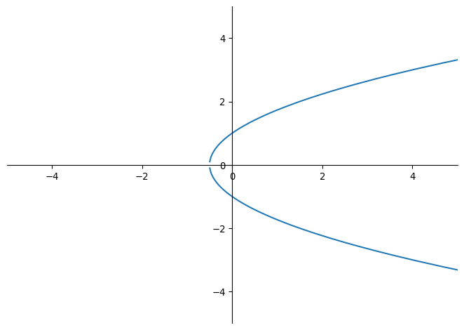
\begin{align*} 1 - c_1 &= 1 - {1 - t^2 \over 1 + t^2} = {2 t^2 \over 1 + t^2} \\ y &= {s_1 \over 1 - c_1} = {2t \over 1 + t^2} {1 + t^2 \over 2 t^2} = {1 \over t} \\ x &= {c_1 \over 1 - c_1} = {1 - t^2 \over 1 + t^2} \cdot {1 + t^2 \over 2 t^2} = {1 - t^2 \over 2t^2} \\ &= {1 \over 2t^2} - {1 \over 2} = {y^2 \over 2} - {1 \over 2} \end{align*}
x is a quadratic polynomial in y, so trivially the figure formed is a parabola. Technically it is missing the point where y = 0 ~ (t = \infty), and this is not a circumstance where using a higher c_n would help. It is however, similar to the situation where we allow o_1(\infty) = -1, and an argument can be made to waive away any concerns one might have.
Ellipse (|\varepsilon| < 1)
Ellipses are next. The simplest fraction between zero and one is 1/2, so for \varepsilon = 1/2,
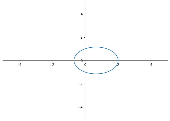
\begin{align*} 1 - {1 \over 2}c_1 &= 1 - {1 \over 2} \cdot {1 - t^2 \over 1 + t^2} = {3 t^2 + 1 \over 2 + 2t^2} \\ y &= {s_1 \over 1 - {1 \over 2}c_1} = {4t \over 3t^2 + 1} \\ x &= {c_1 \over 1 - {1 \over 2}c_1} = {2 - 2t^2 \over 3t^2 + 1} \end{align*}
There isn’t an obvious way to combine products of x and y into a single equation. The general form of a conic section is Ax^2 + Bxy + Cy^2 + Dx + Ey + F = 0, so we know that the implicit equation for the curve almost certainly involves x^2 and y^2.
x^2 = {4 - 8t^2 + 4t^4 \over (3t^2 + 1)^2} \qquad y^2 = {16t^2 \over (3t^2 + 1)^2}
Squaring produces some t^4 terms which cannot exist outside of these terms and xy. A linear combination of x^2 and y^2 never includes any cubic terms in the numerator which would appear in xy, so B = 0. Since all remaining terms are linear in x and y, their denominator must appear as a factor in the numerator of Ax^2 + Cy^2, whatever A and C are.
Since the coefficient of t^4 in x^2 is 4, A must be multiple of 3. Through trial and error, A = 3, C = 4 gives:
\begin{align*} 3x^2 + 4y^2 &= {12 - 24t^2 + 12t^4 + 64t^2 \over (3t^2 + 1)^2} \\ &= {12 - 40t^2 + 12t^4 \over (3t^2 + 1)^2} \\ &= {(4t^2 + 12) (3t^2 + 1) \over (3t^2 + 1)^2} \\ &= {4t^2 + 12 \over 3t^2 + 1} \end{align*}
Since the numerator of y has a t, this is clearly some combination of x and a constant. By the previous line of thought, the constant term must be a multiple of 4, and picking the smallest option finally results in the implicit form:
\begin{align*} 4 &= {4(3t^2 + 1) \over 3t^2 + 1} = {12t^2 + 4 \over 3t^2 + 1} \\ {4t^2 + 12 \over 3t^2 + 1} - 4 &= {8 - 8t^2 \over 3t^2 + 1} = 4x \\[14pt] 3x^2 + 4y^2 &= 4x + 4 \\ 3x^2 + 4y^2 - 4x - 4 &= 0 \end{align*}
Notably, the coefficients of x and y are 3 and 4. Simultaneously, o_1(\varepsilon) = o_1(1/2) = {3 \over 5} + i{4 \over 5}. This binds together three concepts: the simplest case of the Pythagorean theorem, the 3-4-5 right triangle; the coefficients of the implicit form; and the role of eccentricity with respect to stereography.
Hyperbola (|\varepsilon| > 1)
As evidenced by the bound on the eccentricity above, hyperbolae are in some way the inverses of ellipses. Since o_1(2) is a reflection of o_1(1/2), you might think the implicit equation for \varepsilon = 2 to be the same, but with a flipped sign or two. Unfortunately, you’d be wrong.
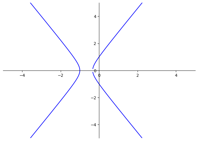
\begin{gather*} \begin{align*} x &= {c_1 \over 1 - 2c_1} = {1 - t^2 \over 3t^2 - 1} \\ y &= {s_1 \over 1 - 2c_1} = {2t \over 3t^2 - 1} \\[14pt] 3x^2 - y^2 &= {3 - 6t^2 + 3t^4 - 4t^2 \over 3t^2 - 1} \\ &= {(t^2 - 3)(3t^2 - 1) \over (3t^2 - 1)^2 } \\ &= {t^2 - 3 \over 3t^2 - 1 } = ... = -4x - 1 \end{align*} \\[14pt] 3x^2 - y^2 + 4x + 1 = 0 \end{gather*}
At the very least, the occurrences of 1 in the place of 4 have a simple explanation: 1 = 4 - 3.
Archimedean Spiral
Arguably the simplest (non-circular) polar curve is r(\theta) = \theta, the unit Archimedean spiral. Since the curve is defined by a constant turning, this is a natural application of the properties of sine and cosine. The closest equivalent in rational polar coordinates is R_1(t) = t. But this can be converted to an implicit form:
\begin{gather*} x = tc_1 \qquad y = ts_1 \\[14pt] x^2 + y^2 = t^2(c_1^2 + s_1^2) = t^2 \\ y = {2t^2 \over 1 + t^2} = {2(x^2 + y^2) \over 1 + (x^2 + y^2)} \\[14pt] (1 + x^2 + y^2)y = 2(x^2 + y^2) \end{gather*}
The curve produced by this equation is a right strophoid with a node at (0, 1) and asymptote y = 2. This form suggests something interesting about this curve: it approximates the Archimedean spiral (specifically the one with polar equation r(\theta) = \theta/2). Indeed, the sequence of curves with parametrization R_n(t) = 2nt approximate the (unit) spiral for larger n, as can be seen in the following video.
Since R necessarily defines a rational curve, the curves will never be equal, just as any stretching of c_n will never exactly become cosine.
Closing
Sine, cosine, and the exponential function, are useful in a calculus setting precisely because of their constant “velocity” around the circle. Also, nearly every modern scientific calculator in the world features buttons for trigonometric functions, so there seems to be no reason not to use them.
We can however be misled by their apparent omnipresence. Stereographic projection has been around for millennia, and not every formula needs to be rewritten in its language. For example (and as previously mentioned), defining the Chebyshev polynomials really only requires understanding the multiplication of two complex numbers whose norm cannot grow, not trigonometry and dividing angles. Many other instances of sine and cosine merely rely on a number (or ratio) of loops around a circle. When velocity does not factor, it will obviously do to “stay rational”.
One of my favorite things to plot as a kid were polar roses, so I was somewhat intrigued to see that they are, in fact, rational curves. On the other hand, their rationality follows immediately from the rationality of the circle (which itself follows from the existence of Pythagorean triples). If I were more experienced with manipulating Chebyshev polynomials or willing to set up a linear system in (way too) many terms, I might have considered attempting to find an implicit form for them as well.
Diagrams created with Sympy and Matplotlib.
Footnotes
This is forgoing the fact that complex derivatives require more care than their real counterparts. It matters slightly less in this case since this function is complex-valued, but has a real parameter.↩︎