Type Algebra and You, Part 3: Combinatorial Types

Isomorphisms through algebra on inducive types.

We know that types have the potential to behave like numbers; the laws for addition, multiplication, and exponentiation are satisfied. However, in the previous post, we also looked at some (potentially dangerous) inductive, self-referential types where arithmetic tries to include the infinite:

• Nat, the natural numbers;
• Any, a chain of Rights followed by a Left wrapped around a value;
• and Stream, an infinite chain of values.

This post will focus on better-behaved types which can be made to resemble familiar objects from algebra.

Geometric Lists

With Stream, there is some difficulty in peeking into the values one contains. We can use its representation from Nat to glimpse one value at a time, but we can’t group an arbitrary number of them into a collection without it on forever.

On the other hand, types like Any which include a sum are allowed to terminate. We can combine a sum and a product to create a new object, a List. Haskell comes with its own implementation, but re-implementing them is a common exercise.

data List a = Null | Cons a (List a)

\begin{gather*} \begin{matrix} \scriptsize \text{A list of X is} & \scriptsize \text{empty} & \scriptsize \text{or} & \scriptsize \text{an X} & \scriptsize \text{and} & \scriptsize \text{a list of X} \\ L(X) = & 1 & + & X & \times & L(X) \end{matrix} \\ \\ \begin{align*} L(X) &= 1 + X \cdot L(X) \\ L(X) - X \cdot L(X) &= 1 \\ L(X) \cdot (1 - X) &= 1 \\ L(X) &= {1 \over 1 - X} \end{align*} \end{gather*}

Unlike with the infinite types where 0 = 1, nothing goes wrong arithmetically. However, the resulting expression doesn’t seem to make sense from the perspective of types. There are no analogues to subtraction or division in type theory. Fortunately, all we need is a trick from calculus, the Taylor series.

\begin{matrix} \scriptsize \text{A list of X is} & \scriptsize \text{empty} & \scriptsize \text{or} & \scriptsize \text{a value of X} & \scriptsize \text{or} & \scriptsize \text{two values of X} & \scriptsize \text{or} \\ L(X) = {1 \over 1 - X} = & 1 & + & X & + & X^2 & + & ... \end{matrix}

This is the geometric series, which appears throughout algebra and analysis. Interestingly, since Stream is more primitive than List, this type includes its supremum, X^\omega.

Something to note about the series is that there is an inherent order to the terms. The 1 term is defined first, then X, then all subsequent ones recursively. This detail also means that the X^2 term is more “ordered” than a typical pair like X \times X.

Another Interpretation

We can equally as well define List in terms of Fix and arithmetic. Instead, the definition is

newtype ListU a b = L (Maybe (a,b))
type List' a   = Fix (ListU a)

\begin{gather*} \hat L(X,Z) = 1 + XZ \\ L(X) = \mathcal Y(\hat L (X,-)) \end{gather*}

The expression 1 + XZ certainly looks like 1 - X, if we let Z = -1. However, we again run into the problem that -1 doesn’t seem to correspond to a type. Worse than that, the actual type we are after is (1 - X)^{-1} = -1 \rightarrow 1 - X.

The latter type seems to resemble a function with -1 on both sides of the arrow. Since the resulting type is intended to resemble a fixed point, we could regard -1 as a sort of “initial type” that gets the list started. Then, we can use the initial definition to replace the occurrence of -1 on the LHS with the entire LHS.

\begin{gather*} (1 - X)^{-1} = -1 ~\rightarrow~ 1 - X \\[8pt] \begin{align*} &\phantom{=} -1 \\[8pt] &\rightarrow 1 \textcolor{red}{-} X \\[8pt] &\rightarrow 1 + X \textcolor{red}{(1 - X)} \\ &= 1 + X \textcolor{blue}{-} X^2 \\[8pt] &\rightarrow 1 + X + X^2 \textcolor{blue}{(1 - X)} \\ &= 1 + X + X^2 + X^3 - X^4 \end{align*} \end{gather*}

This interprets the series as a rewrite rule. Each step is shown before distributing and applying the rule once more. In the limit, when there are no more negative signs to rewrite, we recover the original series.

Convergence

Just like in math, things go wrong when this expression is applied naively. For example, “a list of bools” would seem to have the type

{\texttt{List Bool}} = L(2) \stackrel{?}{=} {1 \over 1 - 2} = -1

If this were true it would mean

• Either () (List Bool) is isomorphic to Void, since 1 + (-1) = 0
• A list of an object X is isomorphic to a function from a list of bools to either a unit or a tuple containing a list of bools and a value of X
  • List a ≅ List Bool -> Either () (List Bool, a)

The first statement is obviously false, since the values Left () and Right [] will always exist. The second statement is dubious. For it to be true, we must imagine values of X can be extracted out of some (possibly infinite) sequence of booleans (the X in the tuple), leaving behind enough information to convert the rest of the list (the List Bool in the tuple), or be exhausted.

The latter argument requires far too much information to be generally true, so I am satisfied with my previous description of -1. It should only show up in the context of a fixed point expression, and is only a valid type in a denominator (the return value of a function from -1).

Iteration

Consider also a list of lists of any type X. Then by iterating lists, it would appear that

\begin{align*} \texttt{List (List a)} &= L(L(X)) \\ &\stackrel{?}{=} {1 \over 1 - {1 \over 1 - X}} = {X - 1 \over X} \end{align*}

If a were Void, then the only possible List to construct is an empty list (L(0) = {1 \over 1 - 0} = 1). Wrapped in another list, the only possible values are those made by repeating this any (natural) number of times. This means that it is itself isomorphic to Nat, and we can write a bijection.

toLists :: Nat -> List (List Void)
toLists Zero     = Null
toLists (Succ x) = Cons Null (toLists x)
-- toLists x = replicate x Null

fromLists :: List (List Void) -> Nat
fromLists Null        = Zero
fromLists (Cons x xs) = Succ (fromLists xs)
-- fromLists = toNat . length

instance Isomorphism Nat (List (List Void)) where
  toA = fromLists
  toB = toLists

  identityA = fromLists . toLists
  identityB = toLists . fromLists

Arithmetically, this implies \omega = 1 + 1 + 1^2 + ... = {1 \over 1 - 1}. More directly, the expression has no Taylor series at 0, and the infinitude of possible values spoils attempting to understand higher order terms. This has big implications, since if we wrap this in another layer of lists,

\texttt{List (List (List a))} = L(L(L(X))) \stackrel{?}{=} {1 \over 1 - {1 \over 1 - {1 \over 1 - X}}} = ... = X

we get back to where we started, which is perfectly absurd. The left-hand side can contain far more Xs than the right-hand side. In other words, by going “past infinity” we have ruined the correspondence between the functor and a series.

A Walk through the Woods

All types thus far have been of a linear form: a List is analogous to a line segment and a Stream is analogous to a ray. All we need to do to go from lists to binary trees is to, for every node, include two sub-structures rather than one.

data Tree2 a = Leaf | Branch a (Tree2 a) (Tree2 a)

\begin{gather*} \begin{matrix} \scriptsize \text{A 2-tree of X is} \\ T_2(X) = & 1 & \scriptsize \text{a leaf} \\ & + & \scriptsize \text{or} \\ & X \times \phantom{1} & \scriptsize \text{a value of X and} \\ & T_2(X) \times \phantom{1} & \scriptsize \text{a left subtree of X and} \\ & T_2(X) \phantom{\times 1} & \scriptsize \text{a right subtree of X} \end{matrix} \\ \\ \begin{align*} 0 &= 1 - T_2(X) + X \times T_2(X)^2 \end{align*} \end{gather*}

Simple enough, but now we have an equation which is quadratic in our functor T_2(X). At this point, we can try to invoke the quadratic formula. Luckily, one of the solutions has a Taylor series which consists of only positive integers, just like the geometric series.

\begin{gather*} a = X, b = -1, c = 1 \\[10pt] \begin{align*} T_2(X) &= {1 - \sqrt{1 - 4X} \over 2X} \\ &= 1 + X + 2X^2 + 5X^3 + 14X^4 + 42X^5 + ... \end{align*} \end{gather*}

The coefficients 1, 1, 2, 5, 14, 42, … are known as the Catalan numbers (OEIS A000108). The OEIS article also pleasantly informs that these count a kind of binary tree on a given number of nodes – one which distinguishes between left and right, as defined by the type.

Rooted binary trees on a particular number of nodes.

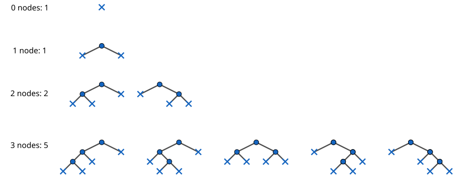
These coefficients have a direct interpretation. If we have three nodes, then there are three locations to place a value of X. In other words, the tree holds an X^3. The coefficient of this term tells us that a value from the type 5 tells us the shape of the nodes on the tree.

Contrast this with the coefficients in the geometric series. They are all 1, telling us that there is only a single shape for a list of a particular size. As consequence, trees are in some sense “larger” than lists. For example, a breadth-first search on a binary tree can collect all values at the nodes into a list. But multiple trees can return the same list, so this is clearly not a bijection. Algebraically, this is because the two series have different coefficients from one another.

Actually Solving the Polynomial

We invoked the quadratic formula to solve the polynomial 1 - T_2(X) + X \times T_2(X)^2, but we haven’t justified the ability to use it. Not only are square roots more suspect than division and subtraction, but the quadratic formula has a choice in sign. Combinatorially, an initial condition determines plus or minus, and the square root is interpreted as a binomial expansion, since \sqrt{1 - X} = (1 - X)^{1/2}.

Naively, the solution seems to have the following interpretation as a type:

\begin{align*} {1 - \sqrt{1 - 4X} \over 2X} &= (1 - (1 - 4X)^{1/2}) \times (2X)^{-1} \\ &= \textcolor{red}{ (1 - ({\scriptsize 1 \over 2} \rightarrow 1-4X)) \times (-1 \rightarrow 2X) } \end{align*}

Compared to the geometric series, this doesn’t make sense. -1 appears in the first term of the product, yet originates from the second term. It doesn’t seem like the iteration can “get started” like it could previously.

We can do some algebra to get terms into the denominator.

\begin{align*} {1 - \sqrt{1 - 4X} \over 2X} &= {2 \over 1 + \sqrt{1 - 4X}} \\ &= \textcolor{red}{ 2 \times (-1 \rightarrow1 + ({\scriptsize 1 \over 2} \rightarrow 1 - 4X) ) } \\[10pt] {1 \over {1 \over 2}(1 + \sqrt{1 - 4X})} &= \textcolor{red}{-1 \rightarrow {\scriptsize 1 \over 2} \times (1 + ({\scriptsize 1 \over 2} \rightarrow 1 - 4X) ) } \end{align*}

The first expression keeps a term in the numerator. Without it, the expression would generate half-integer terms which do not make sense as finite types. To combat this, the second places its reciprocal in the denominator alongside the square root, which appears to describe a second rewrite rule.

While it looks slightly better, I am still unsure whether this result is interpretable. I am also unsure whether it is significant that 1/2 can be expressed as 2^{-1} = (-1 \rightarrow 2). My best guess is that some kind of mutual recursion or alternating scheme is necessary.

Another Solution?

There might still be some hope. The earlier OEIS page mentions that the map which generates the Mandelbrot set has, in the limit, a Taylor series with the Catalan numbers as coefficients.

\begin{gather*} z_{n+1} = z_n^2 + c \\ z \mapsto z^2 + c \\ \\ \begin{matrix} c & \rightarrow & c^2 + c & \rightarrow & (c^2 + c)^2 + c \\ & & & & c^4 + 2c^3 + c^2 + c & \rightarrow & (c^4 + 2c^3 + c^2 + c)^2 + c \\ & & & & & & ... + 5c^4 + 2c^3 + c^2 + c \\ & & & & & & ... \end{matrix} \end{gather*}

The Mandelbrot map is more similar to a type in which leaves, rather than nodes, contain values. We could convert the expression to suit the trees we’ve been working with and to correspond better with the definition of the list.

This interpretation requires special care to work, though. We cannot naively assume that the input i obeys i^2 = -1, since this relationship is not implied by the types.

\begin{gather*} z \mapsto 1 + cz^2 \\[8pt] i \rightarrow 1 + i^2 X = (1 + i^2 X)^i \\ \stackrel{?}{=} (1 - X)^i \\[8pt] \begin{align*} &\phantom{=} 1 \textcolor{red}{-} X \\[8pt] &\rightarrow 1 + X \textcolor{red}{(1 - X)^2} \\ &= 1 + X \textcolor{blue}{-} 2 X^2 + X^3 \\[8pt] &\rightarrow 1 + X + 2 X^2 \textcolor{blue}{(1 - X)^2} + X^3 \\ &= 1 + X + 2 X^2 - 3 X^3 + 2 X^4 \end{align*} \end{gather*}

Doing so appears to work initially, but turns out to produce the series for (1 - X)^{-2}, not (1 - X)^i.

Other Trees

The OEIS article for the Catalan numbers also mentions that the sequence counts “ordered rooted trees with n nodes, not including the root”. In this kind of tree, a node has any number of children rather than just two.

We can construct this type of tree by as the product of a value at the node and the node’s children (possibly none, but themselves trees), called the subforest. A forest is just a list of trees. This defines trees and forests in a mutually recursive way that easily lends itself to algebraic manipulation.

Haskell’s Data.Graph agrees with the following definition

data Tree a = Node a (List (Tree a))
type Forest a = List (Tree a)

\begin{gather*} \begin{matrix} \scriptsize \text{A tree of $X$ is} & \scriptsize \text{a value of $X$} & \scriptsize \text{and} & \scriptsize \text{a forest of $X$} \\ T(X) = & X & \times & F(X) \end{matrix} \\ \begin{matrix} \scriptsize \text{A forest of $X$} & \scriptsize \text{is} & \scriptsize \text{a list of trees of $X$} \\ F(X) & = & L(T(X)) \\ & = & {1 \over 1-T(X)} \\ & = & {1 \over 1-X \times F(X)} \end{matrix} \\ \\ \begin{align*} (1 - X \times F(X)) \times F(X) = 1 \\ -1 + F(X) - X \times F(X)^2 = 0 \\ 1 - F(X) + X \times F(X)^2 = 0 \end{align*} \end{gather*}

The resulting equation for F(X) is the same as the one featured earlier for binary trees, so we know that it generates the same series.

\begin{align*} F(X) = T_2(X) &= {1 - \sqrt{1 - 4X} \over 2X} \\ &= 1 + X + 2X^2 + 5X^3 + 14X^4 + 42X^5 + ... \end{align*}

Binary Bijections

Two finite types were isomorphic when their algebraic equivalents were equal (e.g., Bool ≅ Maybe () because 2 = 1 + 1). Since these structures have the same expression in X, we might assume that the functors are isomorphic with respect to the type X they contain.

For this to actually be the case, there should be a bijection between the two functors, else “isomorphic” ceases to be the proper word. With a bit of clever thinking, we can consider the left (or right) children in a binary tree as siblings, and construct functions that reframe the nodes accordingly.

An example of the correspondence between binary trees and “bushes”, or general trees. A root is shown for the latter to make it better resemble a tree. Leaves and empty subforests not shown.

treeToForest :: Tree2 a -> Forest a
treeToForest Leaf           = Null
treeToForest (Branch x l r) =
  Cons (Node x (treeToForest r)) (treeToForest l)

forestToTree :: Forest a -> Tree2 a
forestToTree Null                  = Leaf
forestToTree (Cons (Node x fs) ns) =
  Branch x (forestToTree ns) (forestToTree fs)

instance Isomorphism (Tree2 a) (Forest a) where
  toA = forestToTree
  toB = treeToForest

  identityA = forestToTree . treeToForest
  identityB = treeToForest . forestToTree

A weaker equality applies in combinatorics: two generating functions are equal if their coefficients are equal. If a closed algebraic expression is known, then it is sufficient to compare them. Instead, we have “generating functors”, which satisfy the same algebraic equation, have the same coefficients as a series, and most strongly, are isomorphic in the sense that they have a bijection.

Ternary and Larger-order Trees

Even though the general tree structure used above encompasses ternary trees, strictly ternary trees have a bit less freedom. In a general tree, a subtree can only appear further along a list of children if all prior elements of the list are filled. On the other hand, in ternary trees, subtrees can occupy any of the three possible positions.

If the binary trees functor satisfy a quadratic, then it stands to reason that ternary trees should satisfy a cubic. And they do:

data Tree3 a = Leaf3 | Node3 a (Tree3 a) (Tree3 a) (Tree3 a)

\begin{gather*} \begin{matrix} \scriptsize \text{A 3-tree of X is} \\ T_3(X) = & 1 & \scriptsize \text{a leaf} \\ & + & \scriptsize \text{or} \\ & X \times \phantom{1} & \scriptsize \text{a value of X and} \\ & T_3(X) \times \phantom{1} & \scriptsize \text{a left subtree of X and} \\ & T_3(X) \times \phantom{1} & \scriptsize \text{a center subtree of X} \\ & T_3(X) \phantom{\times 1} & \scriptsize \text{a right subtree of X} \end{matrix} \\ \\ 0 = 1 - T_3(X) + X \times T_3(X)^3 \end{gather*}

We can solve a cubic with the cubic formula, but it yields a result which is less comprehensible than the one for binary trees.

\begin{gather*} T_3^3 + p T_3 + q = 0 \\ p = -1/X, q = 1/X \\ \\ \begin{align*} T_3(X) &= \sqrt[3]{- {1 \over 2X} + \sqrt{{1 \over 4X^2} - {1\over 27X^3}}} + \sqrt[3]{- {1 \over 2X} - \sqrt{{1 \over 4X^2} - {1\over 27X^3}}} \\ &= {1 \over X}\left( \sqrt[3]{- {X^2 \over 2} + \sqrt{{X^4 \over 4} - {X^3 \over 27}}} + \sqrt[3]{- {X^2 \over 2} - \sqrt{{X^4 \over 4} - {X^3\over 27}}} \right) \\[10pt] &= 1 + X + 3X^2 + 12X^3 + 55X^4 + 273X^5 +... \end{align*} \end{gather*}

The coefficients here are enumerated by OEIS A001764, which doesn’t have a name. Cube roots now feature prominently in the generating functor. This expression is much too large for me to attempt rewriting in “functional” form. WolframAlpha refuses to calculate the series from this expression within standard computation time. Sympy gives an almost-correct series, but which has unsimplified roots of i and has half-integer powers of X.

A series better-suited to computation, based on angle trisection, is adapted from the OEIS here:

T_3(X^2) = {2 \over X \sqrt{3}} \cdot \sin \left( {1\over 3}\arcsin \left(3\cdot{X\sqrt {3} \over 2} \right) \right)

This expression invokes not only irrationals, but trigonometric functions, which are even harder (if not impossible) to understand as types. The situation gets even worse for higher-order trees, where no algebraic formula for the solutions exists. Without being sure how to interpret the simplest case with only square roots, I am unsure whether this has implications for rewrite rules.

Closing

This hardly scratches the surface of constructible datatypes. As a final example, a list which could include pairs as well as singletons of X is counted by the Fibonacci numbers:

data FibList a = NullF | Single a (List a) | Double (a,a) (List a)

\begin{gather*} \begin{matrix} F(X) = 1 + X \times F(X) + X^2 \times F(X) \end{matrix} \\ \\ \begin{align*} 1 &= F(X) - X \cdot F(X) - X^2 \cdot F(X) \\ 1 &= F(X) \cdot (1 - X - X^2) \\ F(X) &= {1 \over 1 - X - X^2} \\ &= 1 + X + 2 X^2 + 3 X^3 + 5 X^4 + ... \end{align*} \end{gather*}

However, I do not feel that it is useful to continue plumbing for types to express as a series. At this basic level, there are still mysteries I am not equipped to solve.

I am the most interested in generalizing rewrite rule-style types. The presence of the square root seems almost opaque. Even the similar Mandelbrot set rule doesn’t cooperate with the “recursive” interpretation of -1. This rule is given in terms of the variable z, but my goal is to is to give an intermediate meaning to -1, not to introduce intermediate “dummy” variables.

I am also interested in extending these ideas to bifunctors (polynomials in multiple variables) and bi-fixes (fixing multiple terms at once, which admittedly the binary tree does already). Perhaps I may explore these ideas in the future.

Tree diagrams made with GeoGebra.

Links

• Haskell/Zippers (from Wikibooks)
  • Another formal manipulation: using the derivative operator on algebraic datatypes. Since the Taylor series is defined in terms of derivatives, there may be a completely type-theoretical characterization that doesn’t rely on “borrowing ideas” from calculus.
• Generating functions for generating trees (paper from ScienceDirect)
  • This paper references enumerates structures by rewrite rules. It also presents a zoo of combinatorial objects and their associated generating functions.