\begin{align*} dk &= \begin{pmatrix}0 & 2 & 0\\0 & 3 & 0\\1 & 0 & 1\end{pmatrix} = \textcolor{red}{\begin{pmatrix}-1 & 0 & 2\\0 & 0 & 3\\1 & 1 & 1\end{pmatrix}}\begin{pmatrix}0 & 0 & 0\\0 & 1 & 0\\0 & 0 & 3\end{pmatrix}\textcolor{blue}{\begin{pmatrix}-1 & 2 / 3 & 0\\1 & -1 & 1\\0 & 1 / 3 & 0\end{pmatrix}} \\ c &= \begin{pmatrix}1 & 2 & 0\\0 & 4 & 0\\0 & 1 & 1\end{pmatrix} = \textcolor{red}{\begin{pmatrix}-1 & 0 & 2\\0 & 0 & 3\\1 & 1 & 1\end{pmatrix}}\begin{pmatrix}1 & 0 & 0\\0 & 1 & 0\\0 & 0 & 4\end{pmatrix}\textcolor{blue}{\begin{pmatrix}-1 & 2 / 3 & 0\\1 & -1 & 1\\0 & 1 / 3 & 0\end{pmatrix}} \\ w &= \begin{pmatrix}1 & 4 & 0\\0 & 7 & 0\\0 & 2 & 1\end{pmatrix} = \textcolor{red}{\begin{pmatrix}-1 & 0 & 2\\0 & 0 & 3\\1 & 1 & 1\end{pmatrix}}\begin{pmatrix}1 & 0 & 0\\0 & 1 & 0\\0 & 0 & 7\end{pmatrix}\textcolor{blue}{\begin{pmatrix}-1 & 2 / 3 & 0\\1 & -1 & 1\\0 & 1 / 3 & 0\end{pmatrix}} \end{align*}
12 Pentagons, Part 3
Exploring even more symmetries based on the 12 pentagons condition.
This is the third part in an investigation into answering the following question:
A soccer ball is a (roughly spherical) figure made of pentagons and hexagons, each meeting 3 at a point. [T]here are 12 pentagons…how many hexagons can there be?
The first post in the series proved the 12 pentagons portion and investigated (dodecahedral) Goldberg polyhedra. The second post investigated tetrahedral Goldberg polyhedra as well as other tetrahedral solutions. Yet more unconventional solutions are presented below.
Combinatorics of Goldberg-Coxeter Operators
In the first post, we established that a solution figure S has feature counts which are parametrized entirely by F_6:
S = \begin{pmatrix} v \\ e \\ f \end{pmatrix} = \begin{pmatrix} 2F_6 + 20 \\ 3F_6 + 30 \\ F_6 + 12 \end{pmatrix} = \begin{pmatrix} 2 \\ 3 \\ 1 \end{pmatrix} F_6 + \begin{pmatrix} 20 \\ 30 \\ 12 \end{pmatrix}
In the last post, it was discovered that certain solutions cannot be created easily from seed polyhedra in a polyhedron viewer. This prompts the question of how to calculate the vertex, edge, and face counts without acquiring them from the output of such a program. Fortunatelly, each of the simple GC operators (dk, c, and w) has a combinatoric matrix form1.
\underset{ \text{Class I} }{ c = \begin{pmatrix} 1 & 2 & 0 \\ 0 & 4 & 0 \\ 0 & 1 & 1 \end{pmatrix} } \quad \underset{ \text{Class II} }{ dk = \begin{pmatrix} 0 & 2 & 0 \\ 0 & 3 & 0 \\ 1 & 0 & 1 \end{pmatrix} } \quad \underset{ \text{Class III} }{ w = \begin{pmatrix} 1 & 4 & 0 \\ 0 & 7 & 0 \\ 0 & 2 & 1 \end{pmatrix} }
These operators are labelled with the classes of Goldberg polyhedra they construct when applied to the dodecahedron.
- dkD = tI = GC(1, 1)
- cD = GC(2, 0)
- wD = GC(2, 1)
It’s worth noting again that dk alternates between producing Class I and Class II solutions.
Diagonalization
tk is the square of the dk operator. Unlike it, it preserves solution class. Powers of a matrix are more readily expressed when the matrix is diagonalized. Diagonalizing each of these operators shows that they have something in common.
All of these operators share the same eigenvectors, which can be seen in the columns of the left outer matrix and rows of the right outer one. This means that composition of these operators only modifies the diagonal matrix, specifically the upper-left and lower-right eigenvalues.
Some of these eigenvectors have special interpretations:
- The left eigenvector (1, -1, 1) (right matrix, middle row) always has eigenvalue 1.
- This means that the operation does not change the Euler characteristic.
- The left eigenvector (3, -2, 0) (right matrix, top row), when applied to general polyhedra, corresponds to the edges and vertices added by the operation:
- In dk, this vector has eigenvalue 0, forcing 3V = 2E, i.e., all vertices to have degree 3.
- In c and w, this vector has eigenvalue 1. These operators only add degree-3 vertices.
The (right) eigenvector (2, 3, 1), deserves special consideration. It happens to be the same as the F_6-dependent component of S. Its eigenvalue is different for the three operators – 4 in the case of c, 3 in the case of dk, and 7 in the case of w. In all three cases, these coincide with the norm of the GC parameters:
\begin{gather*} dkD = GC(1, 1) \longrightarrow \|1 + 1u\| = 1^2 + 1 \cdot 1 + 1^2 = 3 \\ cD = GC(2, 0) \longrightarrow \|2 + 0u\| = 2^2 + 2 \cdot 0 + 0^2 = 4 \\ wD = GC(2, 1) \longrightarrow \|2 + 1u\| = 2^2 + 2 \cdot 1 + 1^2 = 7 \end{gather*}
Call this number T = \|a + bu\| = a^2 + ab + b^2. We know that integers of this form are never congruent to 2 (mod 3). Conveniently, this matches with the upper-left eigenvalue. Assuming for the sake of argument that this is true, it implies something interesting: the GC operators produced from T are (combinatorially) closed under composition. This captures all powers of a given T, as well as products between it and other possible Ts.
However, this combinatorial view misses some of the picture, since some feature counts can be shared between two different classes at once. This comes down to the existence of chiral pairs. For example, ww = (2, 1) \circ (2, 1) = (5, 3), but ww’ = (2, 1) \circ (1, 2) = (7, 0).
This doesn’t affect hexagon counts, so it means we can characterize the possible numbers given a certain T:
\begin{align*} g_T S &= g_T \left( \begin{pmatrix} 2 \\ 3 \\ 1 \end{pmatrix} F_6 + \begin{pmatrix} 20 \\ 30 \\ 10 \end{pmatrix} + \begin{pmatrix} 0 \\ 0 \\ 2 \end{pmatrix} \right) \\ &= T \begin{pmatrix} 2 \\ 3 \\ 1 \end{pmatrix} F_6 + T \begin{pmatrix} 20 \\ 30 \\ 10 \end{pmatrix} + \begin{pmatrix} 0 \\ 0 \\ 2 \end{pmatrix} \\ &= \begin{pmatrix} T(2F_6 + 20) \\ T(3F_6 + 30) \\ T(F_6 + 10) + 2 \end{pmatrix} \\[8pt] F'_6 &= T(F_6 + 10) - 10 \end{align*}
This demonstrates two things: the initial F_6 count from the choice of seed polygon S matters, and we can use valid values of T to produce a sequence of solutions.
Searching for Other Seeds
The dodecahedron, and by extension dodecahedral solutions, have icosahedral symmetry. Tetrahedral symmetry, a sub-symmetry of this, was exploited in the previous post.
However, there are further sub-symmetries which have not been encountered. For example, some lesser symmetries of the dodecahedron are the vertices under rotation and inversion (dihedral, degree 3) and the faces under rotation and inversion (dihedral, degree 5).
Rather than the typical construction based on paths between pentagons, this section will focus on certain base cases followed by a rudimentary application of the Conway operators above. The particular symmetry group of each figure will be mentioned in each section.
Degenerate Deltahedra
Deltahedra are polyhedra formed by equilateral triangles, a table of which is available on Wikipedia. Equilateral triangles are important since three to five of them can be joined at a convex vertex, and if coplanar arrangements are allowed, up to six. Degree-5 and degree-6 vertices can be dualized or truncated to pentagons and hexagons respectively. Additionally, when dualizing, all of the triangles become degree-3 vertices, producing a solution.
All convex deltahedra besides the tetrahedron and icosahedron contain degree-4 vertices. These vertices pose a problem since their duals are quadrilaterals. However, it’s reasonably easy to “correct” these vertices to a higher degree by selectively raising pyramids on faces (augmenting). This section will focus on the coplanar entries on the table.
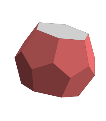
Triangulated Rhombohedron (Dih_3)
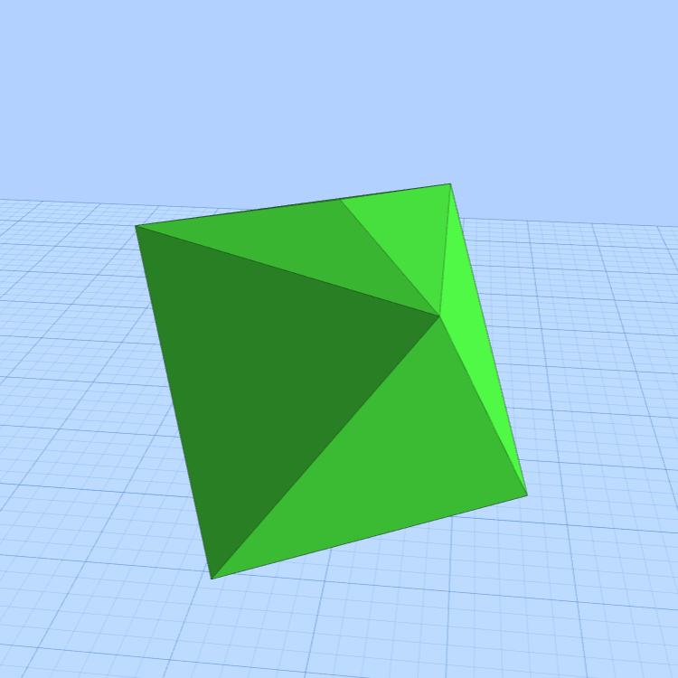
The figure made by cutting the short diagonals of a rhombohedron is one such degree-4 vertex-free deltahedron. It can also be seen as the figure formed by adding two triangular pyramids to opposite faces of an octahedron (a biaugmentation) or as a gyroelongated triangular bipyramid.
Unfortunately, the polyhedron viewer I typically use is unsuitable for visualizing this figure. This viewer supports more operations, and features an operator z which triangulates faces. It produces the desired figure when applied to the cube (which is topologically equivalent to rhombohedra),
Truncating the order-5 vertices produces an eggy-looking figure, It inherits the dihedral symmetry of degree 3 from the vertices of the dodecahedron.
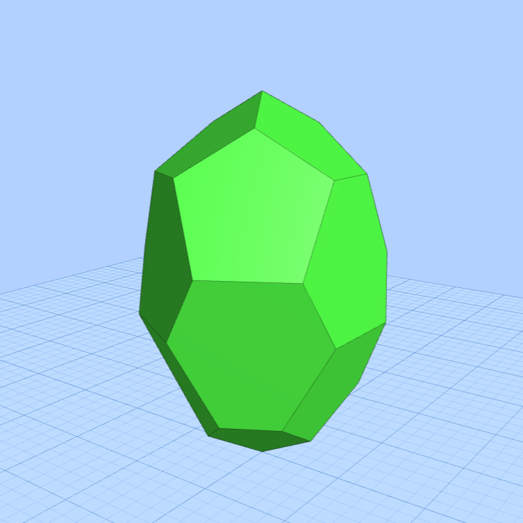
On the opposite pole, blue and red hexagons are exchanged.
| Conway | F_6 | V | E |
|---|---|---|---|
| F | 6 | 32 | 48 |
| F | 38 | 96 | 144 |
| F | 54 | 128 | 192 |
| F | 102 | 224 | 336 |
| F | 134 | 288 | 432 |
| F | 16 T - 10 | 32 T | 48 T |
Base-Triangulated Frustum (Dih_3)
Consider two faces of a figure, one a single equilateral triangle and the other containing four coplanar ones. These two faces can be joined by three triples of triangles in the shape of a half-hexagon. This figure can be seen as an octahedron with three tetrahedra placed around it (a triaugmentation), or as triangulation of the triangular prism.
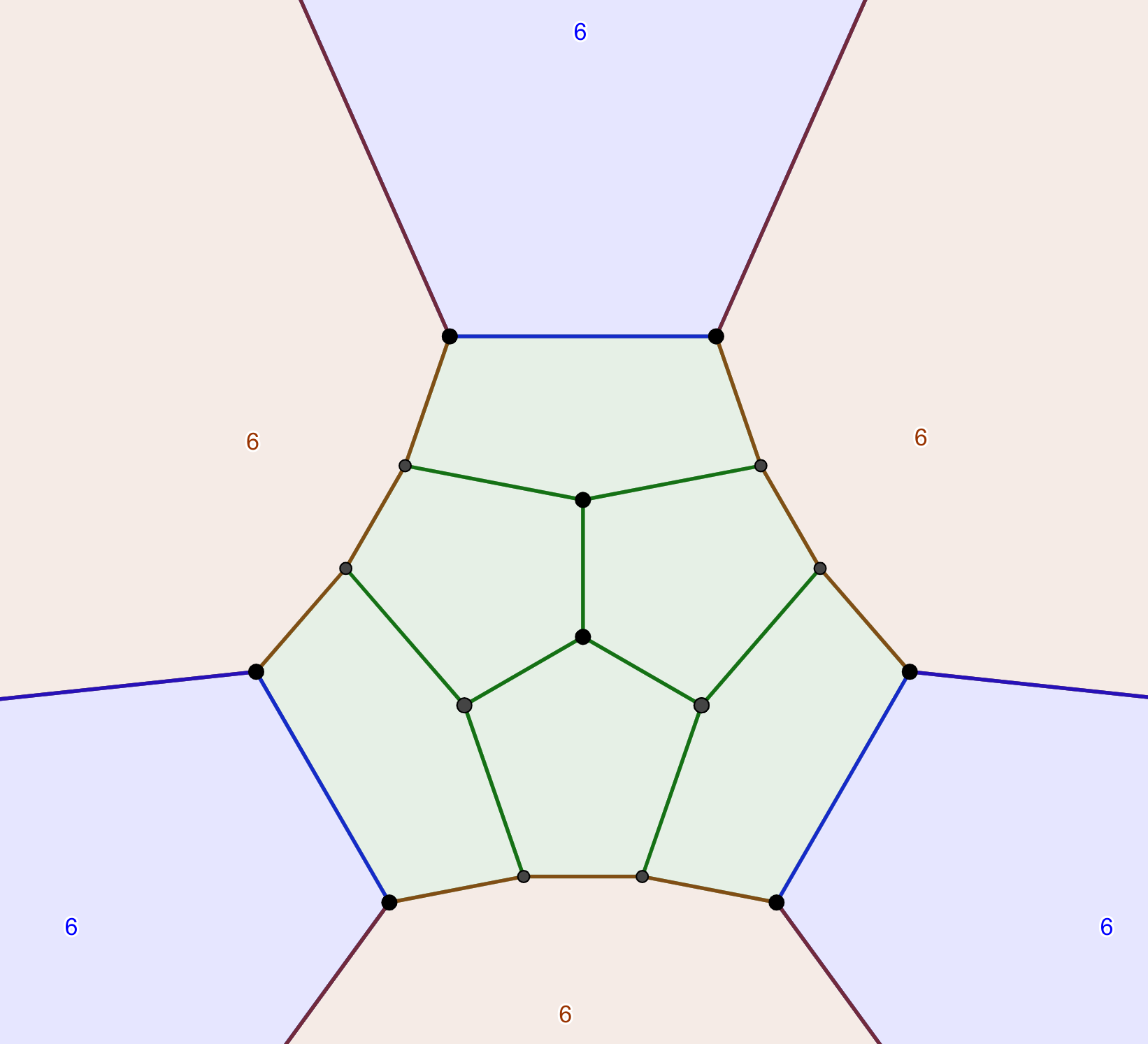
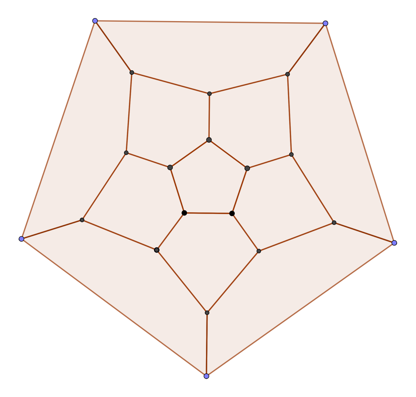
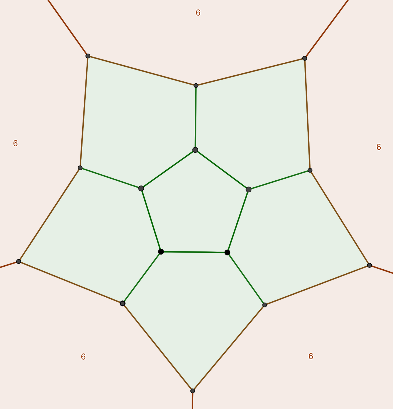
Truncating all vertices except those of degree 3 (t_5 t_6) produces a figure with 8 hexagons and indeed, 12 pentagons. Unfortunately, this figure is not easily constructible from normal seed polyhedra, even in the alternative viewer. However, it is still possible to operate on its projection as a planar graph:
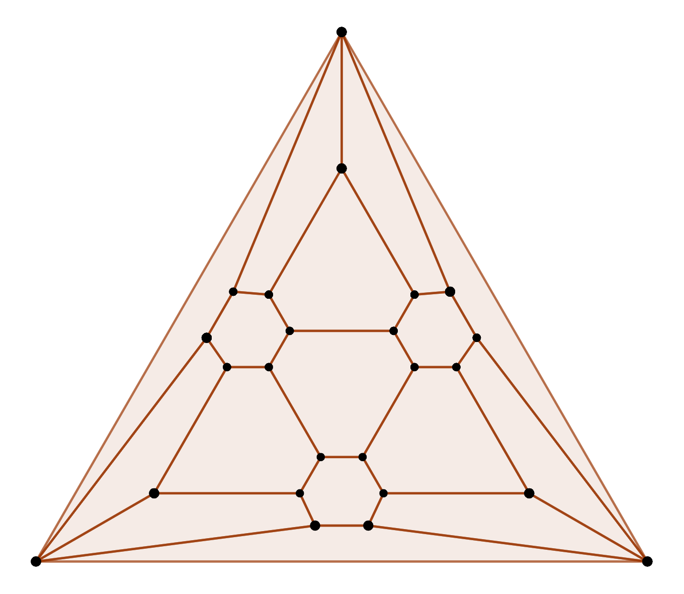
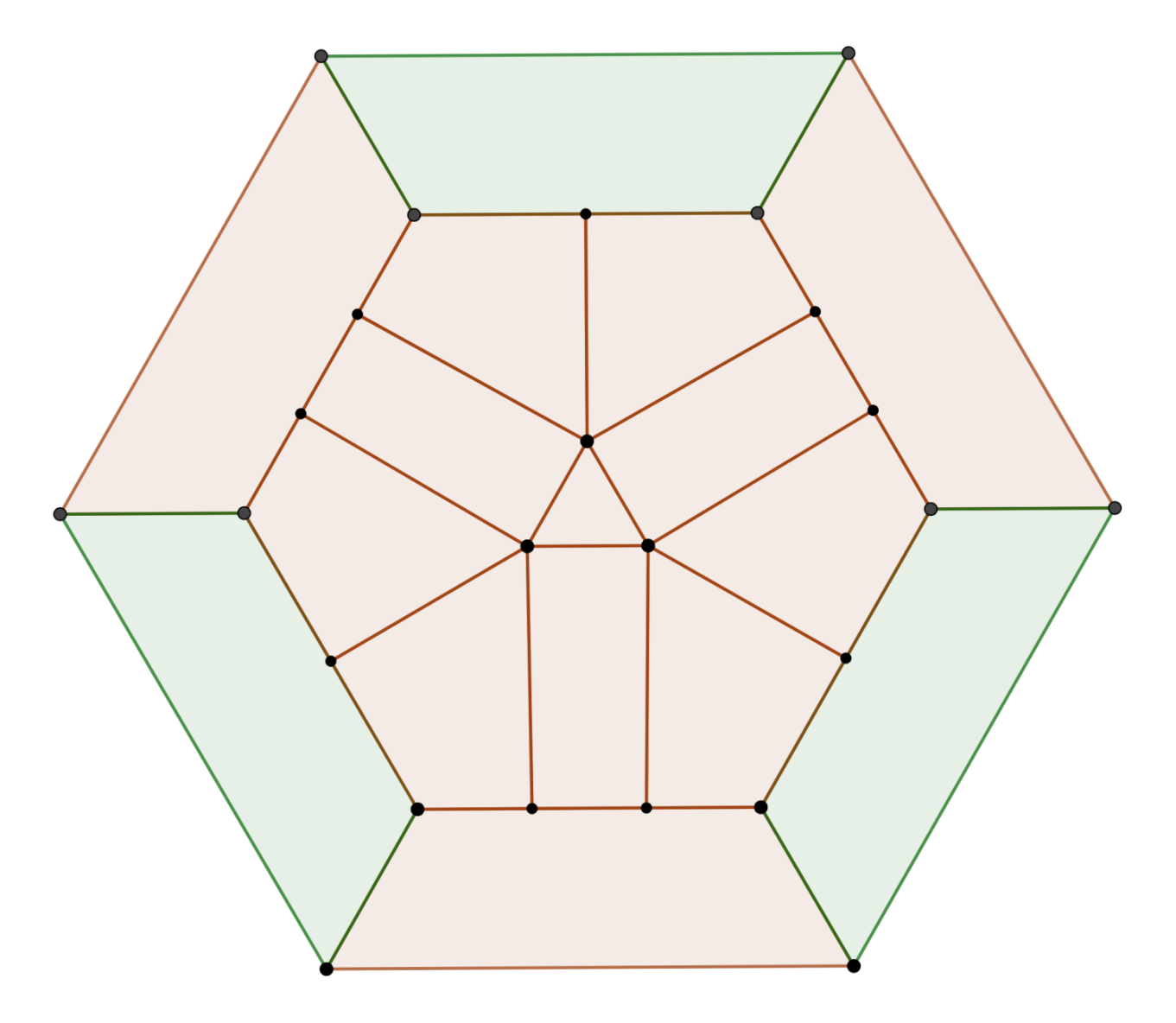
The pentagons gather in groups of 4 and are separated by three bands of hexagons, joined by two hexagons at either end. The symmetry inherited by this figure is also dihedral of degree 3, but centered about a hexagon, rather than (a complex of) pentagons.
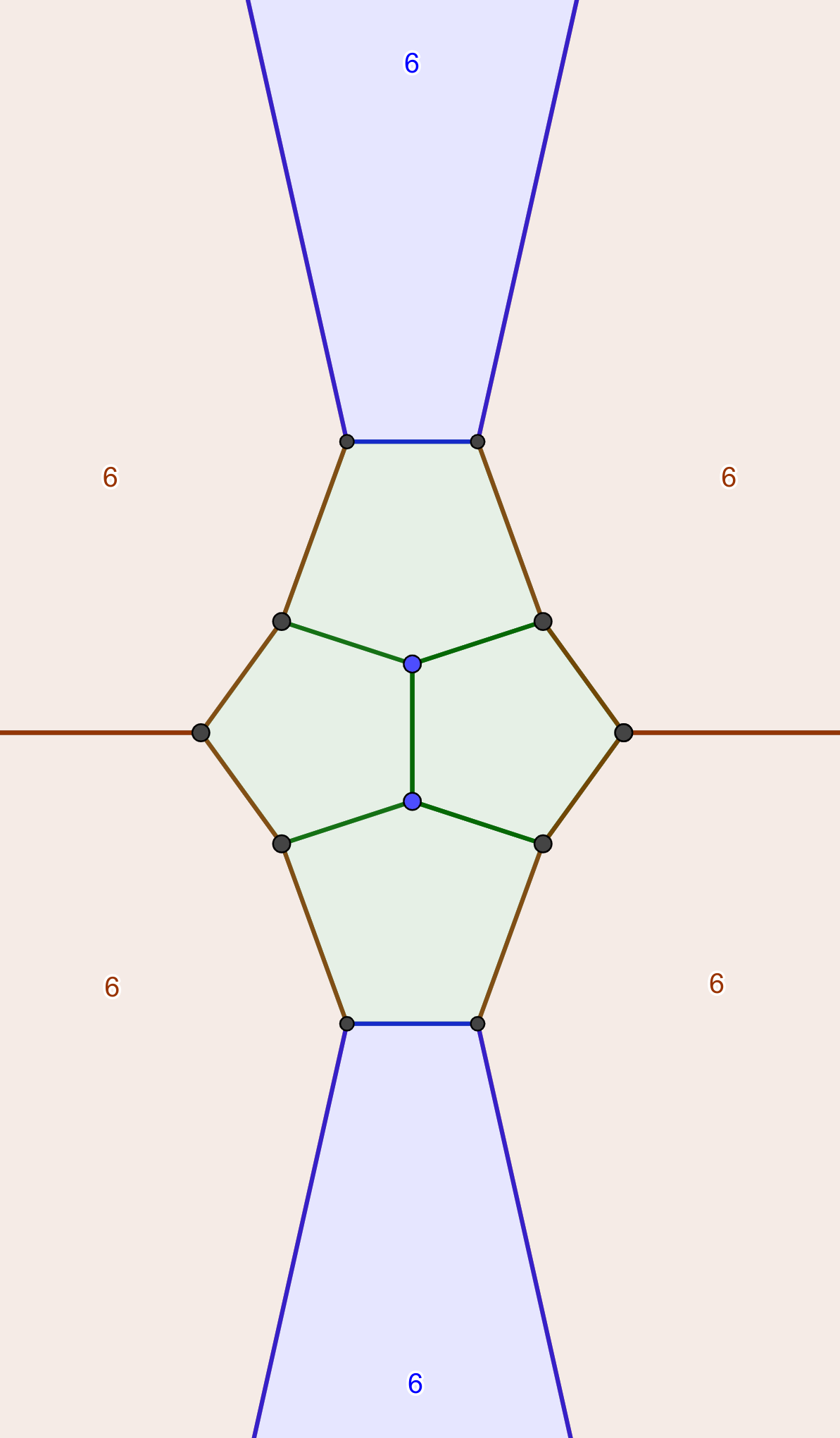
Pentagons in green, band hexagons in red, cap hexagons in blue.
| Conway | F_6 | V | E |
|---|---|---|---|
| F | 8 | 36 | 54 |
| F | 44 | 108 | 162 |
| F | 62 | 144 | 216 |
| F | 116 | 252 | 378 |
| F | 152 | 324 | 486 |
| F | 18 T - 10 | 36 T | 54 T |
Others
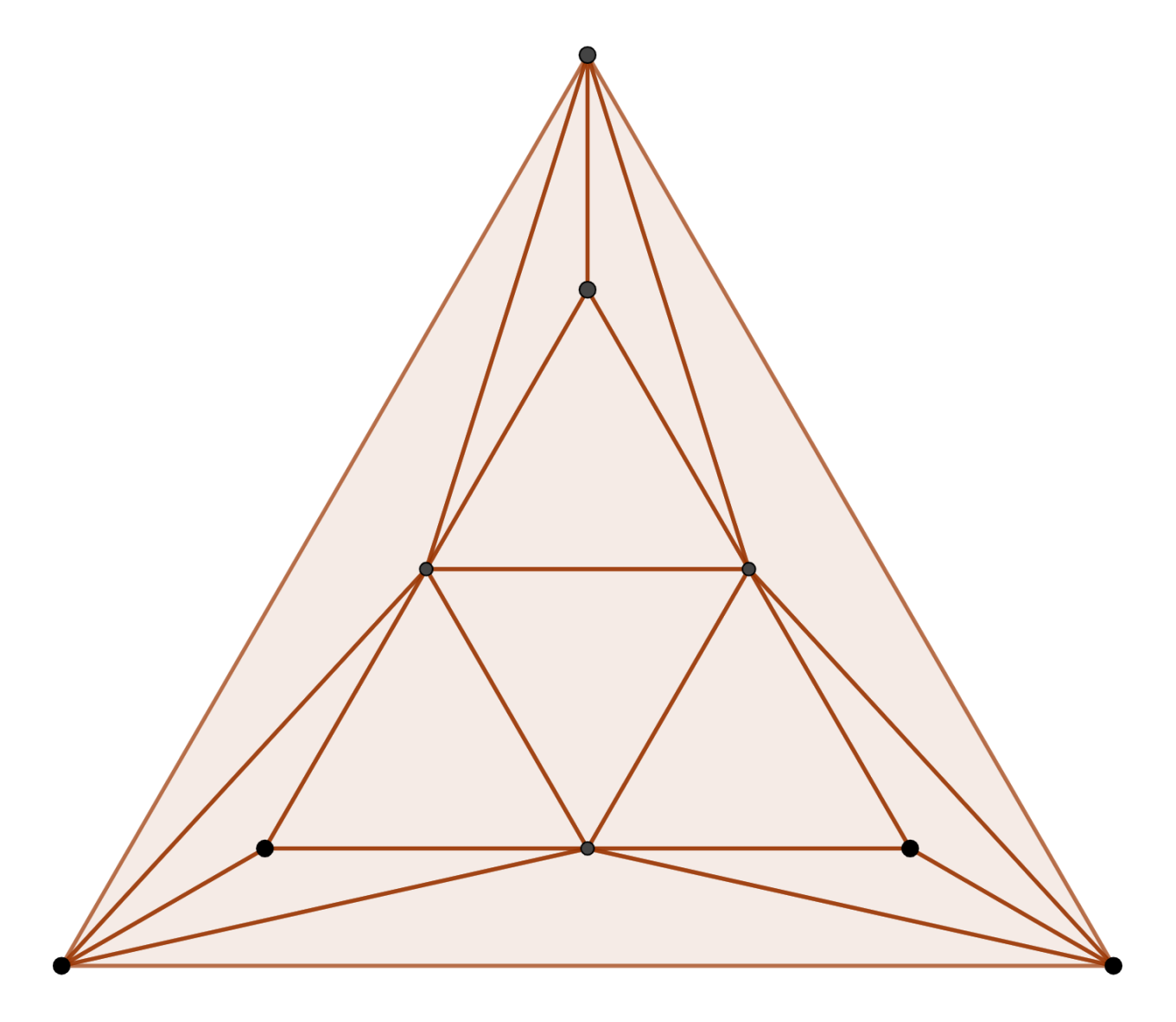
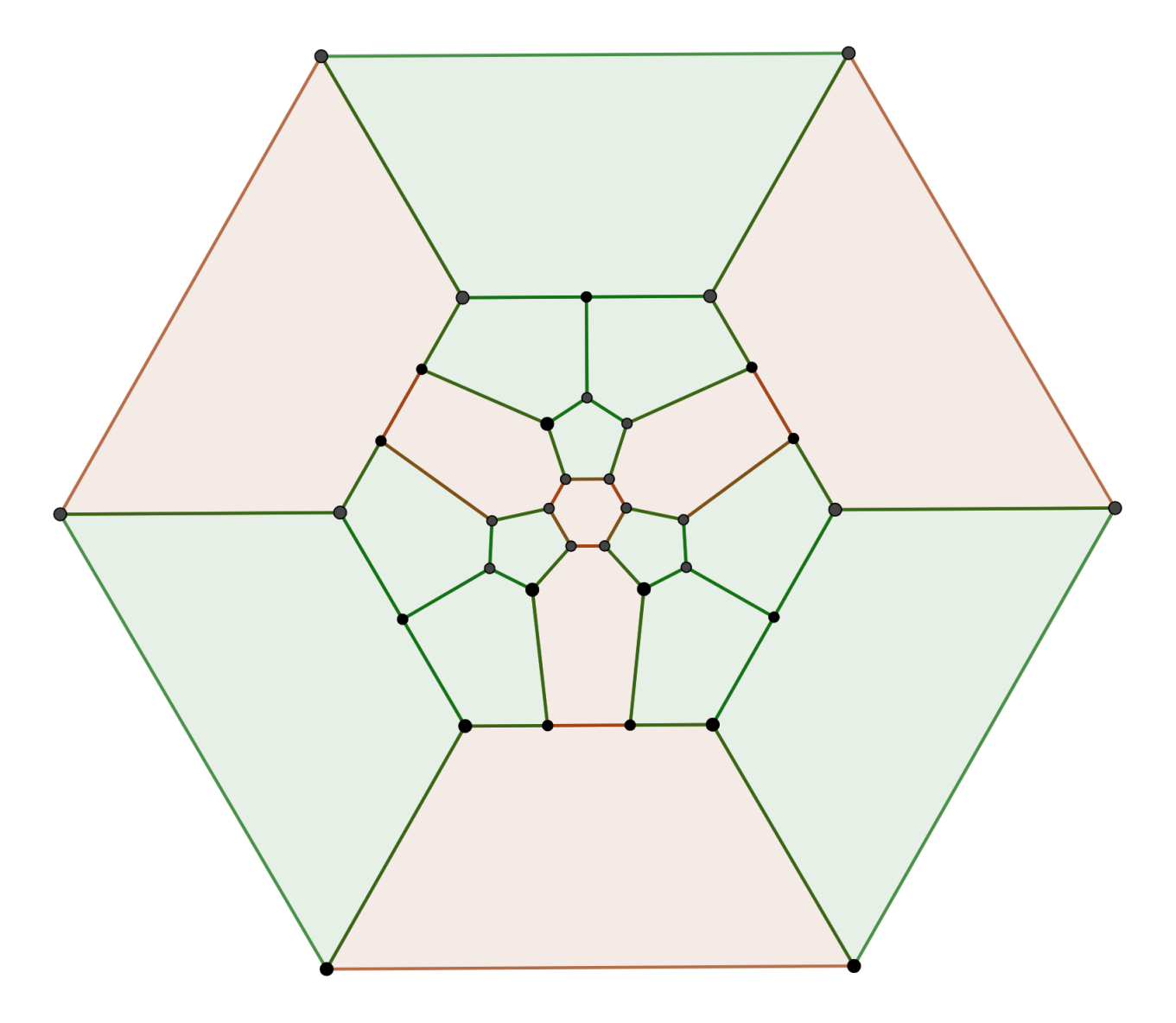
Before their respective truncations, both of these figures of triangles which are compatible with (dual) Goldberg-Coxeter operators. For example, larger triangular subdivisions (in the u_n sense) will also give degenerate deltahedra, Triangular subdivision can add degree-6 vertices, so for the triangulated rhombohedron, an additional order-6 truncation needs to be done. Doing so means t_5 t_6 is applied to either case to form the solution figure.
An example subidivision is shown below. Note how the 3 pentagons at the pole have been separated from another 3 by a triangle of hexagons. I am fairly sure it is possible for mismatched pole configurations to be joined to one another for a more selective subdivision. Other Goldberg-Coxeter operations other than u can also be used; dwd for example connects non-polar pentagons with spirals of hexagons.
F_6 = 60, V = 140, E = 210
F_6 = 114, V = 248, E = 372
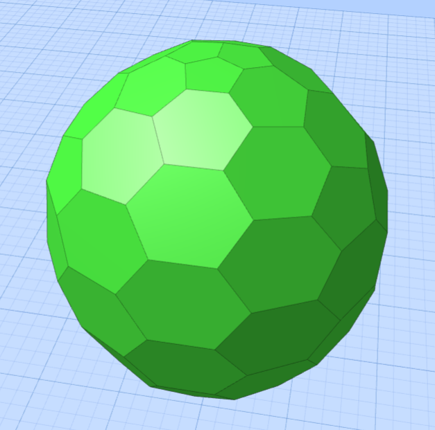
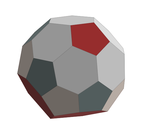
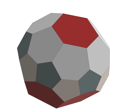
Truncated Trapezohedron (Dih_6)
A trapezohedron is the polyhedral dual of an antiprism. An example is a d10, which is the pentagonal case. Despite the name “n-gonal trapezohedron”, the figure is made entirely from 2n kites with the long edges meeting at points and the short edges meeting with each other.
Truncating the order-n vertices where the long edges of the kites meet produces a truncated trapezohedron, These figures possess two regular n-gonal “caps” separated by a ring of pentagons. In a way, they can be considered as a pentagonal analogue to prisms (quadrilaterals) and antiprisms (triangles).
The dodecahedron itself can be realized as a (order-5) truncated pentagonal trapezohedron (t_5 d A_5), which emphasizes its degree-5 dihedral symmetry. The next largest truncated trapezohedron is the hexagonal case (t_6 d A_6), which contains and 2 hexagons and has dihedral symmetry of degree 6. This is a symmetry beyond that of the icosahedron, but exists due to the symmetry of the hexagon.
| Conway | F_6 | V | E |
|---|---|---|---|
| T_6 | 2 | 24 | 36 |
| t_6dA_6 = T_6 | 26 | 72 | 108 |
| t_6dA_6 = T_6 | 38 | 96 | 144 |
| t_6dA_6 = T_6 | 74 | 168 | 252 |
| t_6dA_6 = T_6 | 98 | 216 | 324 |
| t_6dA_6 = T_6 | 12 T - 10 | 24 T | 36 T |
Medially-Separated Dodecahedron (Dih_5)
As the “truncated pentagonal trapezohedron”, the dodecahedron can be separated into halves along an equator (specifically, along the Petrie polygon). This produces two halves with the pole configuration of the dodecahedron, joined together with hexagons. Organizing the pentagons into two pairs of 6 is similar to the earlier case with the triangulated cube, but with a different arrangement of pentagons. The resultant figure has dihedral symmetry of degree 5.
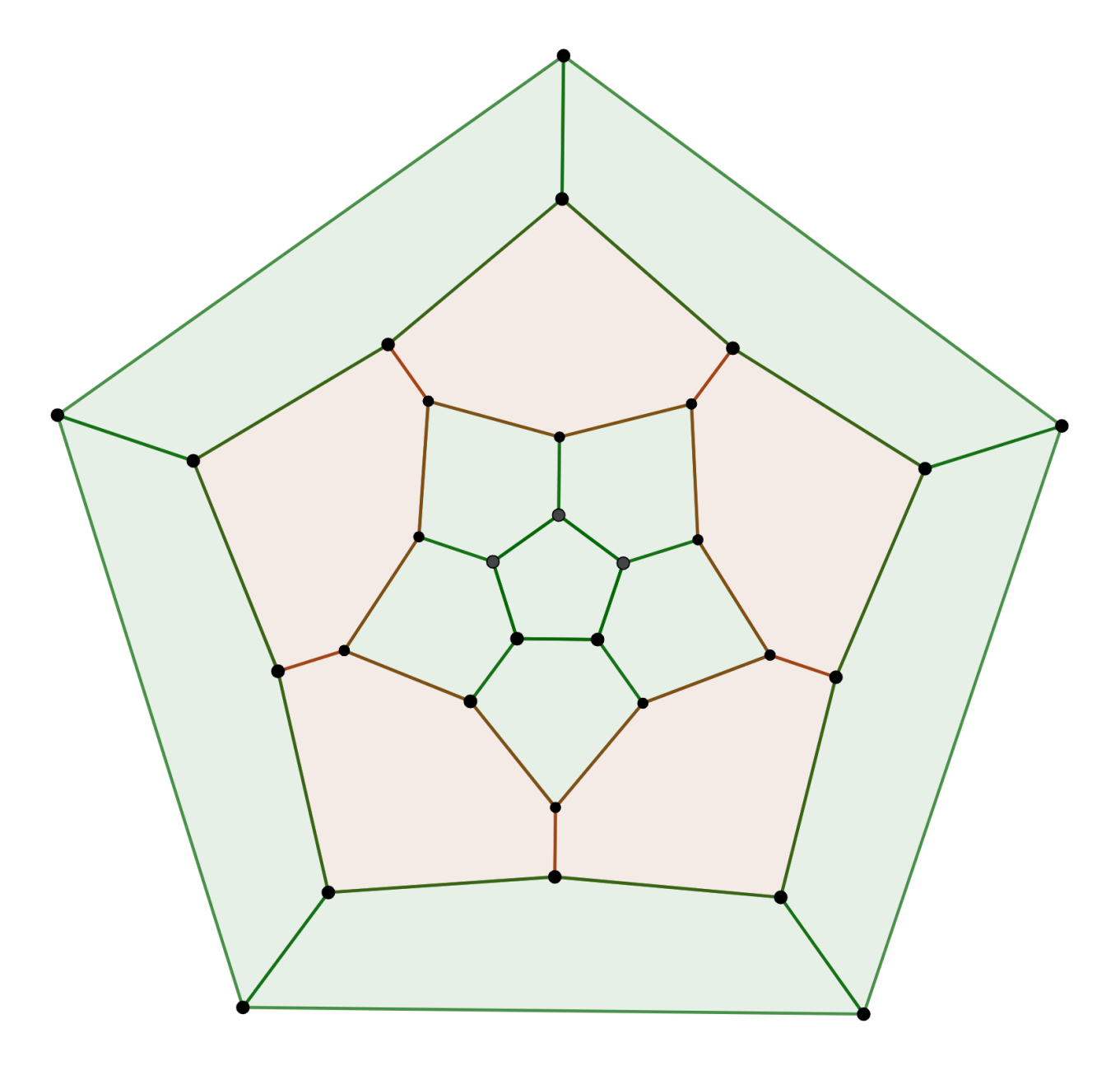
Note how the outer face has been rotated when compared with the dodecahedral graph.
| Conway | F_6 | V | E |
|---|---|---|---|
| D_\pi | 5 | 30 | 45 |
| D_\pi | 35 | 90 | 135 |
| D_\pi | 50 | 120 | 180 |
| D_\pi | 95 | 210 | 315 |
| D_\pi | 125 | 270 | 405 |
| D_\pi | 15 T - 10 | 30 T | 45 T |
Interestingly, this is also the first solution polyhedron with an odd number of faces.
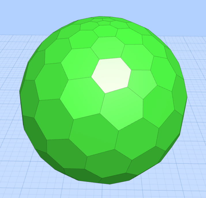
Truncated Gyro-Pyramids (Dih_5, Dih_6)
g, for “gyro”, is a Conway operator I have used, but refused to explain. A gyro-pyramid (i.e., the gyro operator applied to pyramids, [example]](https://levskaya.github.io/polyhedronisme/?recipe=K300gY5)) can roughly be described as a ring of 2n pentagons which alternate in orientation, the tips of which have an additional edge connecting to one of two antipodal endpoints. Truncating these endpoints these adds a face which is the same as the base of the original pyramid, surrounded by hexagons.
Solution polyhedra can be found by examining the pentagonal (t_5 g Y_5) and hexagonal (t_6 g Y_6) cases. The former has dihedral symmetry of degree 5 and the latter has that of degree 6.
| Conway | F_6 | V | E |
|---|---|---|---|
| G_5 | 10 | 40 | 60 |
| t_5gY_5 = G_5 | 50 | 120 | 180 |
| t_5gY_5 = G_5 | 70 | 160 | 240 |
| t_5gY_5 = G_5 | 130 | 280 | 420 |
| t_5gY_5 = G_5 | 170 | 360 | 540 |
| t_5gY_5 = G_5 | 20 T - 10 | 40 T | 60 T |
| Conway | F_6 | V | E |
|---|---|---|---|
| G_6 | 14 | 48 | 72 |
| t_6gY_6 = G_6 | 62 | 144 | 216 |
| t_6gY_6 = G_6 | 86 | 192 | 288 |
| t_6gY_6 = G_6 | 158 | 336 | 504 |
| t_6gY_6 = G_6 | 206 | 432 | 648 |
| t_6gY_6 = G_6 | 24 T - 10 | 48 T | 72 T |
The pentagonal case demonstrates something interesting: an appeal to the partition 12 = 10 + 1 + 1. The similar partition 12 = 5 + 5 + 1 + 1 is unlikely to bear fruit, as an odd number of pentagons cannot alternate up and down.
Japanese Floor Tiling
Tatami are a Japanese traditional style of floor mat, used even today in Japan as an intuitive measure for the surface area of living spaces. A single mat has an aspect ratio of 2:1, but the complexity comes in how they are arranged. Layouts are termed “inauspicious” (不祝儀敷き, fushūgi-jiki) when there are points where four mats meet, while “auspicious” (祝儀敷き, shūgi-jiki) layouts have all mats meet in threes. For a sample of the fascination mathematicians have with these arrangements, you need only search for “tatami” in the OEIS to find dozens of combinatorial sequences.
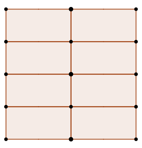
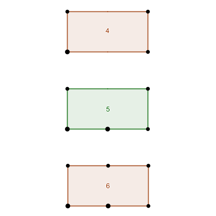
Topologically, each tatami mat in an arrangement can be thought of as either a quadrilateral, a pentagon or a hexagon. Obviously, when considered alone, one mat is a rectangle, as is each mat in the inauspicious layout above. When two mats are affixed to one side of the mat, it becomes a pentagon, as in the auspicious layout above; all 8 mats are pentagons. When done to both sides, it becomes a hexagon.
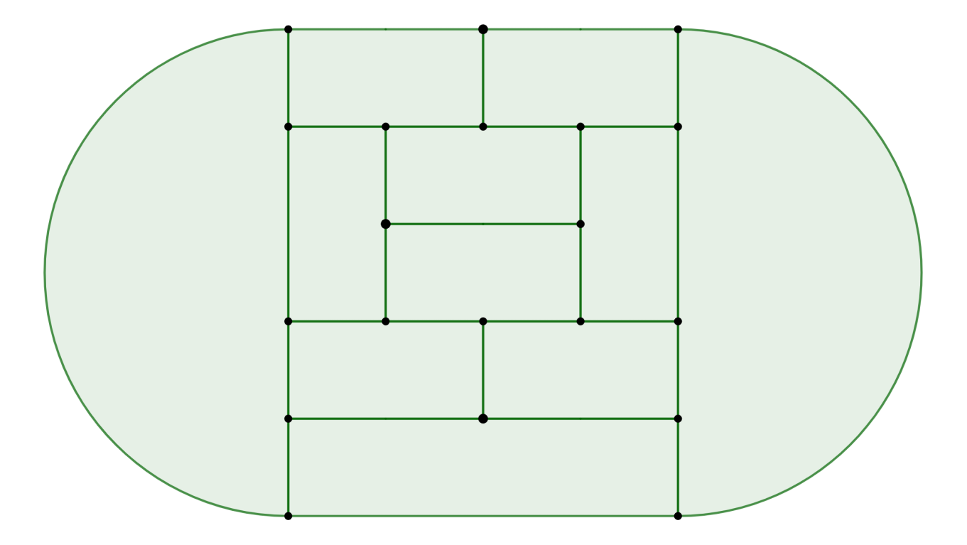
Naturally, the interplay between the latter two elements, as well as the condition that all mats meet in threes has a direct application to the problem at hand. In fact, the graph of the whirl operation on the surface of a cube clearly makes the shape of one of these arrangements (with a half-mat included):


Two things pose a small issue for auspicious floor layouts:
- when interpreted as a graph, the external face very quickly accumulates a large number of edges and
- each of the mats at the corners of the room have a single degree-2 vertex
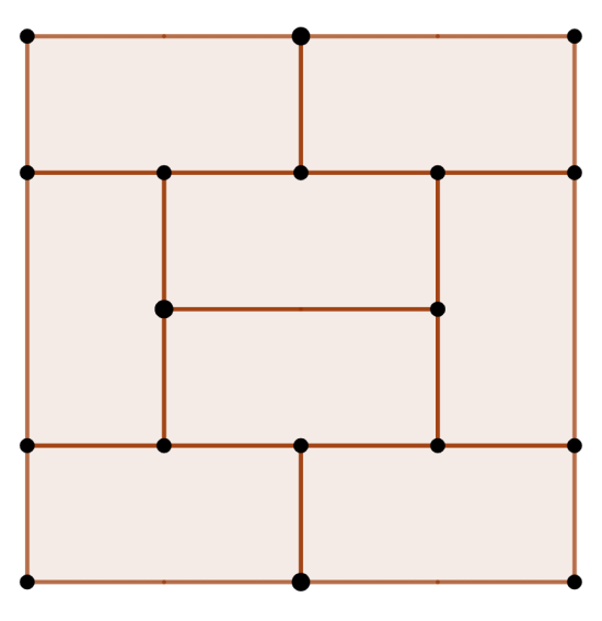
Both of these can be (partially) amended by connecting pairs of corner vertices, which creates additional faces while decreasing the number of edges on the perimeter.
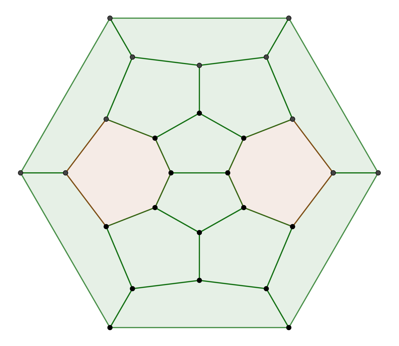
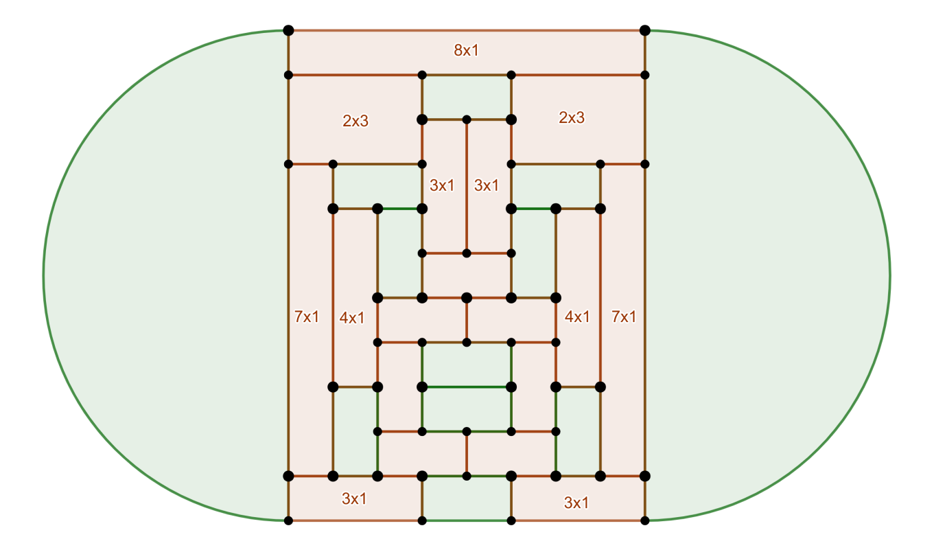
The standard 4x6 auspicious layout is shown below, with corners connected and pentagons/hexagons identified. Next to it is an equivalent graph with a regular hexagon as an outer face. As a 3D figure, it has only three hexagons and degree-3 dihedral symmetry, another odd number.
| Conway | F_6 | V | E |
|---|---|---|---|
| M | 3 | 26 | 39 |
| M | 29 | 78 | 117 |
| M | 42 | 104 | 156 |
| M | 81 | 182 | 273 |
| M | 107 | 234 | 351 |
| M | 13 T - 10 | 26 T | 39 T |
While c and w produce counts which are multiples of 3, dk somewhat strangely generates 29 and 107, which are both prime. In fact, up to (dk)^{11}, the values are either prime or semiprime, and up to (dk)^{28}, the values are either 1-, 2-, or 3-, almost primes.
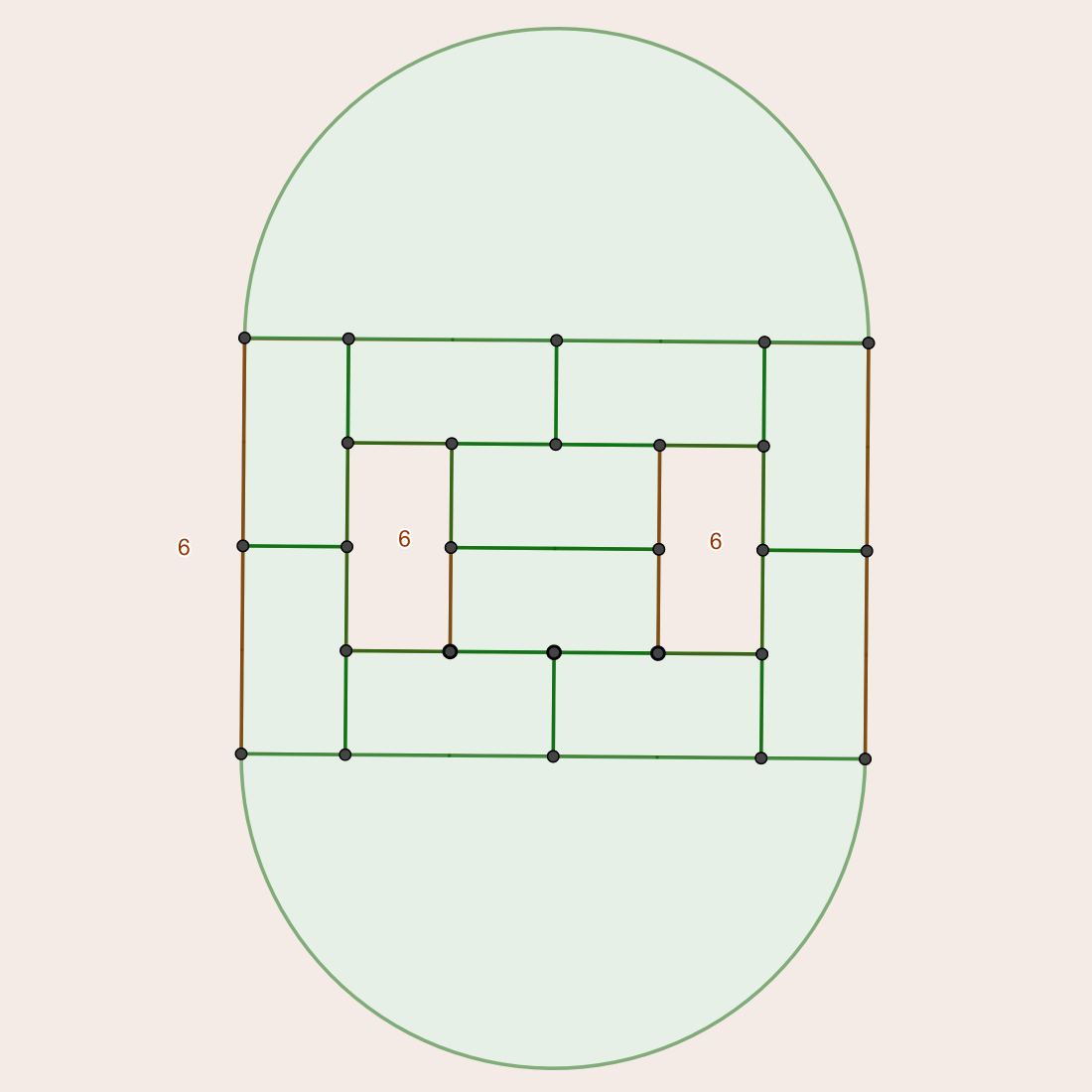
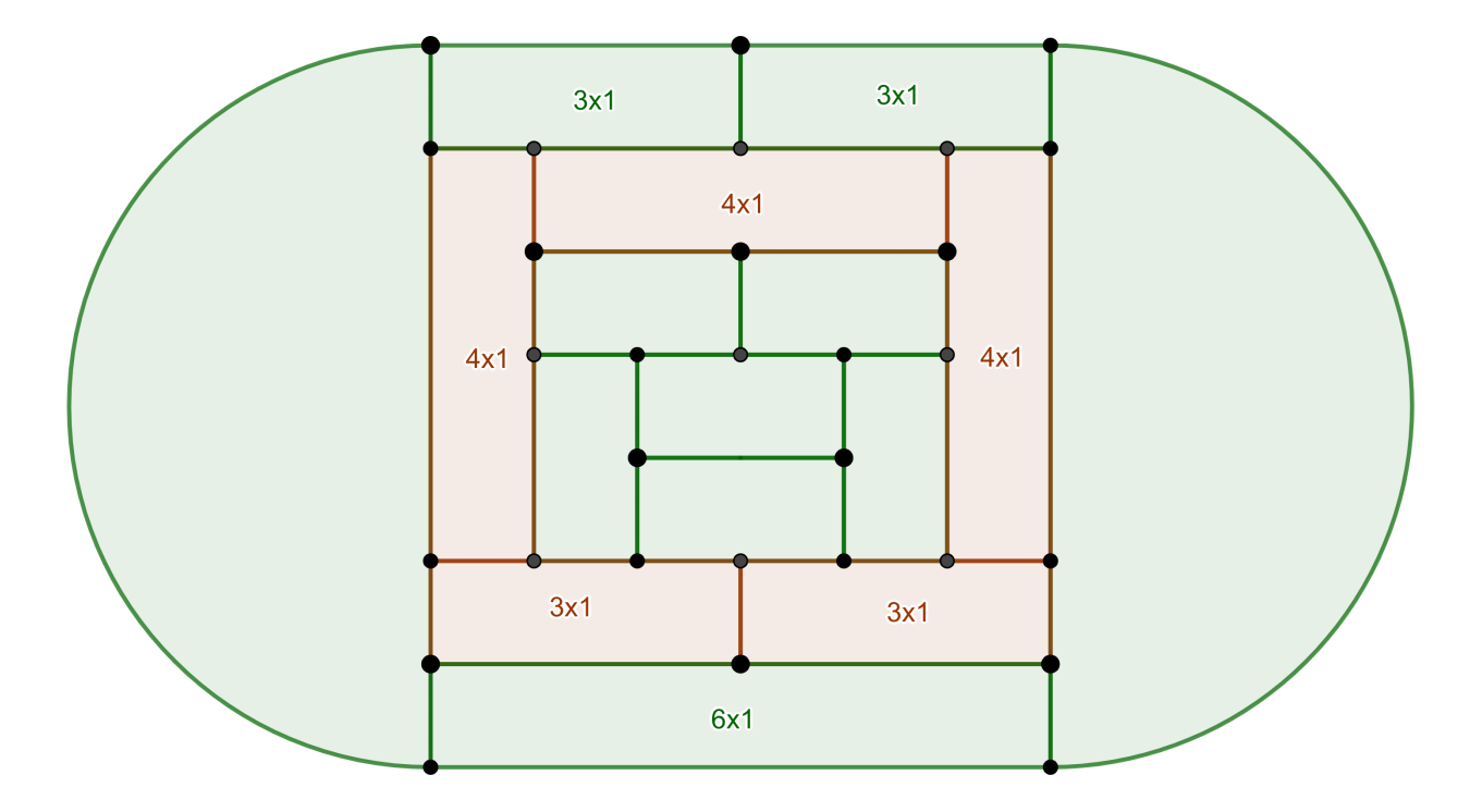
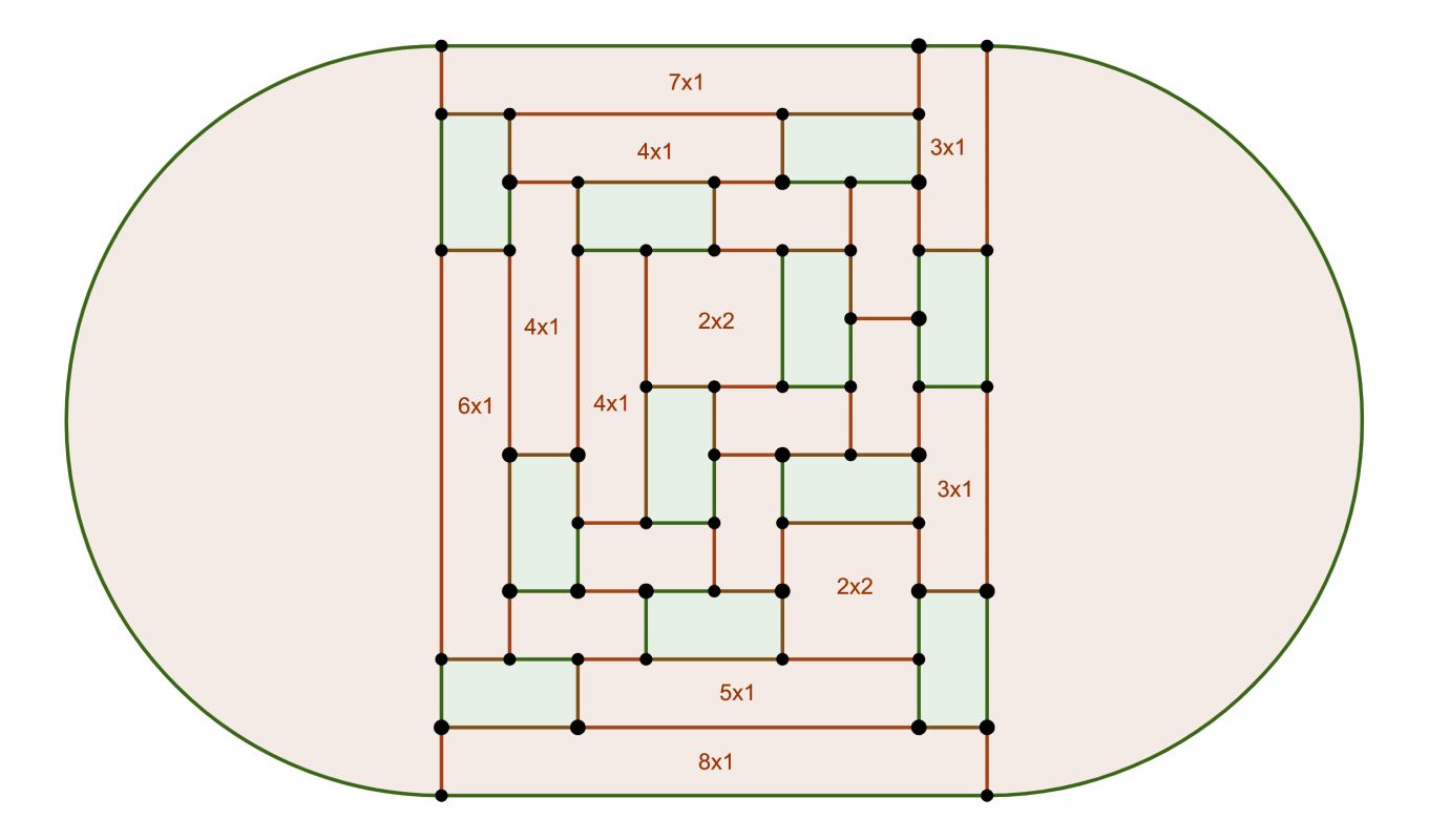
Tatamified Projections
While other rectangular tatami arrangements contain either too few or too many edges, graphs of solution polyhedra can be produced by using mats with nonstandard aspect ratios (and connecting corners as necessary).
Some of these are shown below:
Final Tabulation
The solutions examined have been collected in the table below.
| Symmetry | Classification | F_6 | Example Values |
|---|---|---|---|
| Icosahedral | Dodecahedral Goldberg | 10 T - 10 | 20, 30, 60, 80, 110, 120, 150, 180, 200, 240 |
| Tetrahedral | Tetrahedral Goldberg Antitruncations | 2 T - 14 | 4, 10, 12, 18, 24, 28, 36, 40, 42, 48 |
| GC(Antitruncations)* | T' \left(2 T - 4\right) - 10 | 32, 46, 50, 56, 70, 74, 78, 88, 92, 102 | |
| Class I Edge-preserving | 4 \left(n + 1\right)^{2} - 12 | 4, 24, 52, 88, 132, 184, 244, 312, 388, 472 | |
| GC(Edge-preserves) | T' \left(4 \left(n + 1\right)^{2} - 2\right) - 10 | 32, 46, 88, 92, 116, 126, 158, 172, 176, 214 | |
| Dih_3 | Triangulated Rhombohedron | 16 T - 10 | 6, 38, 54, 102, 134, 182, 198, 246, 294, 326 |
| Triangular Frustum | 18 T - 10 | 8, 44, 62, 116, 152, 206, 224, 278, 332, 368 | |
| Tatamihedron | 13 T - 10 | 3, 29, 42, 81, 107, 146, 159, 198, 237, 263 | |
| Dih_5 | Medially-separated Dodecahedron | 15 T - 10 | 5, 35, 50, 95, 125, 170, 185, 230, 275, 305 |
| Truncated Pentagonal Gyropyramid | 20 T - 10 | 10, 50, 70, 130, 170, 230, 250, 310, 370, 410 | |
| Dih_6 | Truncated Hexagonal Trapezohedron | 12 T - 10 | 2, 26, 38, 74, 98, 134, 146, 182, 218, 242 |
| Truncated Hexagonal Gyropyramid | 24 T - 10 | 14, 62, 86, 158, 206, 278, 302, 374, 446, 494 |
Here are a few hexagon counts from the table, sorted in ascending order:
2, 3, 4, 5, 6, 8, 10, 12, 14, 18, 20, 24, 26, 28, 29, 30, 32, 35, 36, 38…
However, keep in mind that this list is not exhaustive. In particular, it may be possible to construct additional entries by applying selective GC operators which preserve certain symmetries, like in the edge-preserving tetrahedral and deltahedron cases.
Some small naturals which do not appear on the list are 1, 7, 9, 11, and 13. Without constructing them, I am unsure whether they can exist. Some possible partitions to consider are 7 = 5 + 1 + 1 (five equatorial and two polar hexagons, Dih_5) and 11 = 3 + 3 + 3 + 1 + 1 (three hexagons along three lines of longitude or three triangles of hexagons pointing toward a pole, Dih_3).
Closing
Despite the Goldberg-Coxeter construction for dodecahedra being well-known, the 12 pentagons rule applies to a much broader class of polyhedra. In fact, due to the GC construction, any polyhedron satisfying its conditions can be expanded and twisted into larger and larger solutions, which are far out of the way of ordinary soccer balls.
Polyhedron images were generated using polyHédronisme and Dr. Andrew J. Marsh’s polyhedron generator. Nets and graphs were created with GeoGebra. Other images were retrieved from Wikimedia and belong to their respective owners.
Footnotes
These matrices can be derived by closely observing the vertex, edge, and face counts of a figure before and after applying the operator. Gather the feature counts of the tetrahedron, dodecahedron, and icosahedron into a matrix.
\begin{gather*} f \begin{pmatrix} | & | & | \\ T & D & I \\ | & | & | \end{pmatrix} = f \begin{pmatrix} 4 & 20 & 12 \\ 6 & 30 & 30 \\ 4 & 12 & 20 \end{pmatrix} = \begin{pmatrix} | & | & | \\ fT & fD & fI \\ | & | & | \end{pmatrix} \\ f = \begin{pmatrix} | & | & | \\ fT & fD & fI \\ | & | & | \end{pmatrix} \begin{pmatrix} 4 & 20 & 12 \\ 6 & 30 & 30 \\ 4 & 12 & 20 \end{pmatrix}^{-1} \end{gather*}
This matrix is invertible, and the feature counts for fT, fD, and fI can be acquired from a viewer implementing the operator f.↩︎