Stereographic Hyperspheres

How do you explicitly describe n-dimensional spheres?

In the first post of this series, we explored a definition of quaternions and their application to rotation in three dimensions. In doing so, we used stereography to define a point on the 2-sphere, i.e., one whose coordinates satisfy x^2 + y^2 + z^2 = 1.

It’s easy to extend this implicit equation to higher-dimensional spheres (or hyperspheres). A point (x_0, x_1, x_2, ... x_n) is on a unit hypersphere in n+1-dimensional Euclidean space if

x_0^2 + x_1^2 + x_2^2 + ... + x_n^2 = 1

This follows naturally from the definition of the sphere as the locus of points which all have the same distance to the origin. Since this has an implicit equation, there’s a natural question: how do we parameterize hyperspheres?

Guidance from Lower Dimensions

Because points on the sphere are constrained by an equation, there is one fewer degree of freedom than a general point in the space they occupy. Hence, a sphere in n+1-dimensional space is itself n-dimensional, and is termed an n-sphere.

As a basic example, the complex unit circle is a 1-sphere in the 2-dimensional complex plane:

o(t) = {1 + it \over 1 - it} = {1 - t^2 \over 1 + t^2} + i{2t \over 1 + t^2}

The explicit map for the 2-sphere is similar; we have two parameters and have two “nonreal”s i and j, which turned out to be quaternions.

o_2(s, t) = {1 + is + jt \over 1 - is - jt} = {1 - s^2 - t^2 \over 1 + s^2 + t^2} + i{2s \over 1 + s^2} + j{2t \over 1 + t^2}

These are valid constructions because division works for both complex numbers and quaternions. But the ability to divide isn’t very common in higher dimensions, so without justification, we can’t extend it and hope the math works out.

Topological Insights

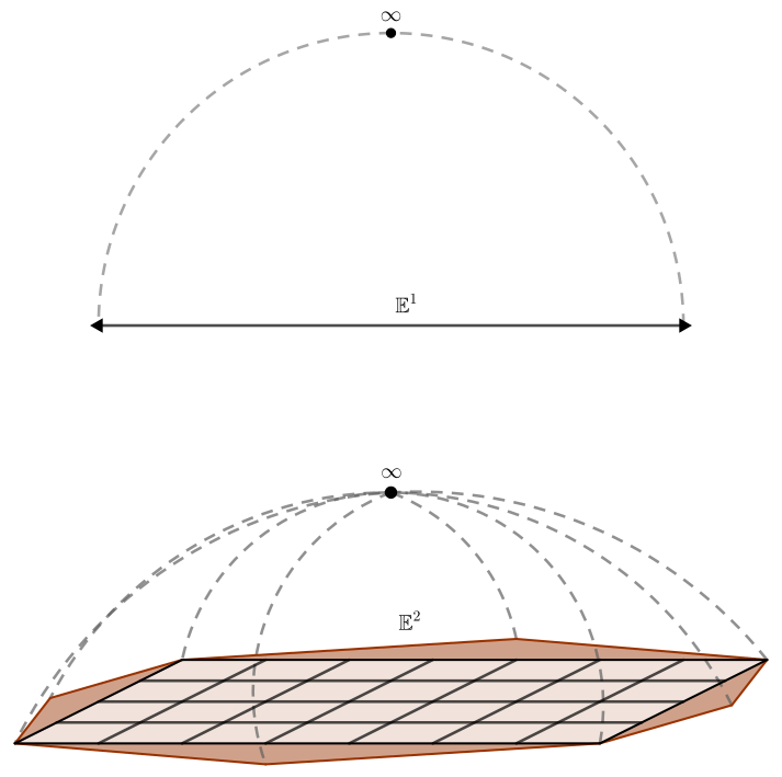
In above equation for a circle, we assign values to t from a number line, a 1-dimensional Euclidean space. More precisely, the line is the imaginary axis it in the numerator. We also include an extra point “at infinity”. This same point is approached regardless of whether t is negative or positive, and “closes” the circle.

\begin{align*} o(\infty) &\approx {1 + i\infty \over 1 - i\infty} \approx {-\infty \over \infty} \approx -1 \\ o(-\infty) &\approx {1 - i\infty \over 1 + i\infty} \approx {\infty \over -\infty} \approx -1 \end{align*}

For (2-)spheres, a similar statement holds true. Rather than a line, we range over the imaginary plane is + jt, a 2-dimensional Euclidean space. If one or both of the parameters s or t has a value of “infinity”, then they seem to describe the same point.

\begin{align*} o_2(s, \infty) &\approx {1 + is + j\infty \over 1 - is - j\infty} \approx {\infty \over -\infty} \approx -1 \\ o_2(\infty, t) &\approx {1 + i\infty + jt \over 1 - i\infty - jt} \approx {\infty \over -\infty} \approx -1 \end{align*}

In both expressions, the point at infinity contains no “nonreals” like i or j. In another sense, the real space is the extra dimension into which the sphere extends as a surface.

Topologically, this description of the resulting space is called the one-point compactification. In other words, the circle is the one-point compactification of the line, and in general, an n-sphere is the one-point compactification of Euclidean n-space.

\mathbb{E}^{n} \cup \{ \infty \} \cong S^n

One-point compactification of 1- (top) and 2- (bottom) dimensional Euclidean space. Both spaces extend indefinitely in the indicated directions before joining up at \infty.

Invariance of Dimension

The topological definition seems to imply that our construction shouldn’t care about how many dimensions are in the space. In fact, when constructing the 2-sphere, all we cared about was that i and j anti-commute to get cancellation.

Geometric algebra gives some tools to generalize this argument to higher dimensions. In an n-dimensional algebra, we have unit vectors {\vec e_0}, {\vec e_1}, ..., {\vec e_{n-1}} and the following properties:

• Scalars and vectors can be added and multiplied together, and all possibilities comprise the algebra
• The product of a unit vector with itself is a scalar, generally chosen among -1, 0, or 1
• Scalars commute, but the product of two different unit vectors anticommutes
  • e.g., {\vec e_0} {\vec e_1} = - {\vec e_1} {\vec e_0}
  • Consequently, the square of the product is the negative of the product of the squares
    • e.g., {\vec e_0} {\vec e_1} {\vec e_0} {\vec e_1} = - {\vec e_0} {\vec e_1} {\vec e_1} {\vec e_0} = - {\vec e_0^2} {\vec e_1^2}
• Division by anything other than scalars is undefined

A consequence is that the square of a general vector \vec v with components {\vec e_k}x_k is a scalar. This can be seen by arranging the components of the product after distributing as a square:

\begin{align*} {\vec v} &= {\vec e_0} x_0 + {\vec e_1} x_1 + ... {\vec e_{n-1}} x_{n-1} = \sum_k {\vec e_k} x_k \\ {\vec v^2} &= (\sum_k^{n-1} {\vec e_k} x_k) (\sum_l^{n-1} {\vec e_l} x_l) = \sum_k^{n-1} \sum_l^{n-1} {\vec e_k} {\vec e_l} x_k x_l \\ &= \underset{\diagdown}{\sum_k^{n-1} {\vec e_k^2} x_k^2} + \underset{◥}{ \sum_k^{n-1} \sum_{l > k} {\vec e_k} {\vec e_l} x_k x_l } + \underset{◣}{ \sum_k^{n-1} \sum_{l < k} {\vec e_k} {\vec e_l} x_k x_l } \end{align*}

Due to anticommutativity, we can cancel the upper and lower triangles, leaving only the diagonal.

\begin{align*} ◣ &= \sum_k^{n-1} \sum_{l < k} {\vec e_k} {\vec e_l} x_k x_l = \sum_k^{n-1} \sum_{k < l} {\vec e_l} {\vec e_k} x_l x_k \\ &= - \sum_k^{n-1} \sum_{l > k} {\vec e_k} {\vec e_l} x_k x_l = - ◥ \\[10pt] &\implies \diagdown + ◥ + ◣ = \diagdown + ◥ - ◥ = \diagdown \end{align*}

To align with the prior examples i and j, we’ll assume that {\vec e_k^2} = -1 for all k. This means that {\vec v}^2 = - ||{\vec v}||, the sum of squares of the extent in each basis (or Euclidean norm).

Being Hyperrational

Finally, we can consider an expression analogous to the one from which we derived the 1- and 2-spheres.

Suppose that a vector and a scalar are added together, as a + {\vec u}. If this point is on a sphere and the scalar component is considered the extent in a new dimension, then the norm of the entire quantity should be

||a + {\vec u}|| = a^2 + ||{\vec u}|| = a^2 - {\vec u}^2 = 1

Now let a vector \vec v range over n-dimensional space. The expression…

{\bm o_n}({\vec v}) = a + {\vec u} = {1 + {\vec v} \over 1 - {\vec v}}

…seems to be a ratio between two distinct quantities with the same norm, since 1^2 - {\vec v}^2 = 1^2 - (-{\vec v})^2. However, it’s ill-defined since there is a vector we can’t divide by in the denominator. Due to the properties of the algebra, we can use a conjugation trick to clear it:

\begin{align*} {1 + {\vec v} \over 1 - {\vec v}} &= \left( {1 + {\vec v} \over 1 - {\vec v}} \right) \left( {1 + {\vec v} \over 1 + {\vec v}} \right) = {(1 + {\vec v})^2 \over (1 - {\vec v})(1 + {\vec v})} \\ &= {1 + 2{\vec v} + {\vec v}^2 \over 1 - {\vec v}^2} \\ &= {1 - ||{\vec v}|| \over 1 + ||{\vec v}||} + {2{\vec v} \over 1 + ||{\vec v}||} = a + {\vec u} \end{align*}

The quantity in the denominator of both components is always a scalar and greater than zero, so there are no concerns about the validity of division. We can also show that the norm of this expression is 1, as desired:

\begin{align*} a^2 - {\vec v}^2 &= 1 \\ \implies \stackrel{\text{Numerator of } a}{(1 + {\vec v}^2)^2} - \stackrel{\text{Numerator of } \vec u}{(2{\vec v})^2} &= \stackrel{\text{Common denominator}}{1 - {\vec v}^2} \end{align*}

This is true no matter how many dimensions \vec v has¹, justifying our earlier abuse of notation.

Inducing an Alternative

The previous topological description of spheres lacks a couple of things:

• It does not make reference to lower-dimensional spheres
• “Points at infinity”, while intuitive, are logically suspect

Fortunately, topology has an alternate description.

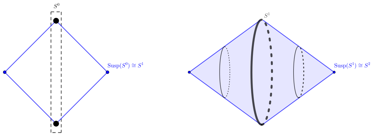
The 0-dimensional sphere is a little bit special. On a number line, there are two points equidistant to the origin, and these comprise the 0-sphere S^0. This can (topologically) be turned into a 1-sphere S^1 (the circle) by an operation called suspension, which connects all points in the space to two new, auxiliary points. Subsequently, we can take the circle and repeat the operation to build the 2-sphere S^2.

Example of suspension of the 0- and 1-spheres, forming the 1- and 2-spheres, respectively. The space is duplicated along the blue lines except at the two blue endpoints.

In general,

\text{Susp}(S^{n-1}) = S^n

Algebraic Suspension

Let’s compare the topological definition with what we have algebraically. We first definied the circle, or 1-sphere as

o(t) = {1 + it \over 1 - it} = {1 - t^2 \over 1 + t^2} + i{2t \over 1 + t^2}

Negating t keeps the real part the same, but negates the imaginary part. So in most cases, where there is an imaginary part, the space looks two discrete points; to wit, a 0-sphere. The remaining two points 1 and -1 are the exception.

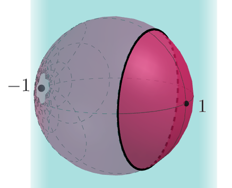
Similarly, when we intersect the 2-sphere with a plane along a line of latitude, the space looks like a 1-sphere except at the two poles, also 1 and -1.

The sphere, as parametrized by {\bm o_2}({\vec v}), being intersected by a plane. The plane is perpendicular to the line connecting -1 and 1 and intersects the sphere in a circle (1-sphere).

Halfway between the two poles, at the equator, the scalar component is 0 and the sphere is a pure vector. For a general sphere, this happens when ||{\vec v}|| = 1:

{\bm o_n}({\vec v}) = {1 - ||{\vec v}|| \over 1 + ||{\vec v}||} + {2{\vec v} \over 1 + ||{\vec v}||} = {1 - 1 \over 1 + 1} + {2 \over 1 + 1}{\vec v} = {\vec v}

In general, this happens when \vec v is a point on a unit sphere of one dimension lower. For the 2-sphere, this is a 1-sphere, which we can easily parametrize using o. Being a unit sphere, all points on it behave similarly to i in that their square is -1. Thus, we can construct an expression for the 2-sphere by replacing i with the vector in question.

\begin{align*} {\vec v} = {\vec w}_1(s) &= {1 - s^2 \over 1 + s^2} e_0 + {2s \over 1 + s^2} e_1 \\[10pt] {\bm \varsigma}_2(s,t) &= {1 + {\vec w}_1(s)t \over 1 - {\vec w}_1(s)t} = {1 - t^2 \over 1 + t^2} + {2t \over 1 + t^2} {\vec w}_1(s) \end{align*}

Just like with o, if t is replaced with -t in the above expression, then the scalar part remains the same, but the vector part (which corresponds to latitudinal circles) is negated. Since the circle is a connected space, we only need one of the two circles this generates, and s must range over [0, \infty]. s, however, ranges over [-\infty, \infty), since that’s the domain of o.

This process can be continued indefinitely – at each stage, \bm \varsigma_n² describes a n-dimensional unit sphere. It can be converted to a pure vector {\vec w}_n by multiplying the scalar component with a new unit vector e_n. In this form, {\vec w}_n^2 = -1 for any n-dimensional algebra³. This provides an inductive construction parallel to the topological one.

\begin{align*} {\vec w}_n(x_0, x_1, ..., x_{n-1}) &= V({\bm \varsigma}_n(x_0, x_1, ..., x_{n-1})) \\ &= \text{Scalar}({\bm \varsigma}_n)e_n + \text{Vector}({\bm \varsigma}_n) \\ {\bm \varsigma}_{n+1}(x_0, x_1, ..., x_{n-1}, x_n) &= {1 + {\vec w}_n(x_0, x_1, ..., x_{n-1})x_n \over 1 - {\vec w}_n(x_0, x_1, ..., n_{n-1})x_n} \\ &= {1 - x_n^2 \over 1 + x_n^2} + {2x_n \over 1 + x_n^2}{\vec w_n} \end{align*}

When the new parameter x_n is 0 or \infty, the vector part collapses, and we get either 1 or -1, the “new points” of the suspension.

\begin{align*} {\bm \varsigma}_{n+1}(..., 0) &= {1 + {\vec w}_n(...)\cdot 0 \over 1 - {\vec w}_n(...) \cdot 0} - {1 \over 1} = 1 \\ {\bm \varsigma}_{n+1}(..., \infty) &\approx {1 + {\vec w}_n(...)\cdot \infty \over 1 - {\vec w}_n(...) \cdot \infty} \approx {\infty \over -\infty} \approx -1 \end{align*}

All spheres but the 0-sphere are connected spaces, so duplicate latitudinal spheres occur in all dimensions greater than 1. Only in dimension 1 are negative numbers required for the expected duplication. More directly, this means that the parameter attached to the 1D case (x_0) ranges over positive and negative numbers, but all others range over only positve numbers.

Multiple Wrappings

One feature of the complex rational circle mentioned in the previous article was that its powers correspond to going around multiple times. Conveniently, a similar fact holds for n-spheres in general.

Starting with the scalar/vector form of the sphere, we can square the sphere and apply the fact that the difference of squares of each part is constant:

\begin{align*} {\bm o}_n &= a + {\vec u} \\ {\bm o}_n^2 &= (a + {\vec u})^2 \\ &= a^2 + {\vec u}^2 + 2a{\vec u} +\textcolor{red}{(0 = a^2 - {\vec u}^2 - 1)} \\ &= 2a^2 - 1 + 2a{\vec u} = 2a(a + {\vec u}) - 1 \\ &= 2a {\bm o_n} - 1 \end{align*}

This gives the familiar recurrence relation…

{\bm o}_n^{m+2} = 2a {\bm o}_n^{m+1} - {\bm o}_n^m

…and thus a sphere can be wrapped around itself any number of times, as given by

{\bm o}_n^m = T_m(a) + U_{m-1}(a){\vec u}

where T and U are the standard Chebyshev polynomials.

Negative Indices

The topological equivalent to this statement is

H_n(S^n) = \Z

More directly, a map from the n-sphere to itself can be characterized by an integer, the degree, and these compose as integers add.

Since this is an integer, there’s the notion of maps in an opposite direction which correspond to negative degrees. This seems to align with the behavior of the exponent m in {\bm o}_n^m. However, we’ve only defined m over positive integers; after all, \bm o_n contains a vector, so we can’t really divide by it.

Fortunately, it’s pretty easy to make sense of this. Since we have a recurrence relation for the powers of the n-sphere, we can extend it backwards to define it over negative indices⁴.

\begin{align*} {\bm o}_n^1 &= 2a {\bm o}_n^{0} - {\bm o}_n^{-1} \\ a + {\vec u} &= 2a - {\bm o}_n^{-1} \\ {\bm o}_n^{-1} &= a - {\vec u} \end{align*}

This actually aligns with what we’d expect according to adding powers, since:

({\bm o}_n^1)({\bm o}_n^{-1}) = (a + {\vec u})(a - {\vec u}) = a^2 - {\vec u}^2 = 1 = {\bm o}_n^0

Degrees and Induction

The inductive case was established by noticing that a vector \vec w lying on a unit sphere behaves similarly to i in that that {\vec w}^2 = -1. We can use the same trick for higher-order wrappings – the only thing that needs changing from the previous article is replacing “real” with “scalar” and “nonreal” with “vector”.

{\bm \varsigma}_n^m = ( c + s { {\vec w}_{n-1}} )^m = T_m(c) + s U_m(c) {\vec w}_{n-1}

Similarly,

\begin{align*} {\bm \varsigma}_n^{-1} &= ( c - s{\vec w}_{n-1} ) \\ ({\bm \varsigma}_n^{1}) ({\bm \varsigma}_n^{-1}) &= ( c + s{\vec w}_{n-1} )( c - s{\vec w}_{n-1} ) \\ &= c^2 - s^2 {\vec w}_{n-1}^2 = c^2 + s^2 = 1 \\ &= {\bm \varsigma}_n^0 \end{align*}

Technically, \bm \varsigma_n is already a higher-degree map when all parameters (besides the one from the base case) are allowed to range over negative numbers. In this case, \bm \varsigma_2^\pm is a degree-2 map, \bm \varsigma_3^\pm is a degree-4 map, and \bm \varsigma_n^\pm is a degree-2^{n-1} map.

De-infinitizing

The degree also gives us the tools to address “points at infinity”. If \vec w_n is a point on the equatorial unit n-1-sphere, then \bm o_n behaves as the identity. But we also know that it squares to -1, and that squaring \bm o_n produces a degree-2 map.

{\bm o}_n({\vec w}_n)^2 = {\vec w}_n^2 = -1

This means that the degree-2 map can be interpreted as collapsing the equator to a single point, the pole -1. The hemi-n-sphere surrounding the antipode 1 gets closed, resulting in the whole n-sphere.

# circle map
s,t = sympy.symbols("s t", real=True)
o = (1 + sympy.I*s) / (1 - sympy.I*s)

# doubled map for finite range
o2 = o**2
o2_real, o2_imag = o2.as_real_imag()

# inductive 2-sphere
sphere_x = o2_real.subs(s,t)
sphere_y = o2_imag.subs(s,t)*o2_real
sphere_z = o2_imag.subs(s,t)*o2_imag

def animate_sphere(filename: str, n=30, interval=80):
  lerp_steps = np.linspace(0, 1, n)
  t_hemisphere = 2**0.5 - 1

  with SympyAnimationWrapper(filename) as animate:
    @animate(len(lerp_steps), interval=interval)
    def ret(fr):
        plt.clf()
        lerp = lerp_steps[fr]

        t_upper = t_hemisphere*(1 - lerp) + 1*lerp
        p = plot.plot3d_parametric_surface(
            sphere_x, sphere_y, sphere_z,
            (s, -1, 1), (t, 0, t_upper),
            xlim=(-1,1), ylim=(-1,1), zlim=(-1,1),
            show=False,
            backend="matplotlib",
        )
        p2 = plot.plot3d_parametric_line(
            sphere_x.subs(t, t_upper), sphere_y.subs(t, t_upper), sphere_z.subs(t, t_upper),
            (s, -1, 1),
            show=False,
            backend="matplotlib",
        )
        p.append(p2[0])
        p.show()

    ret.save()  # type: ignore

animate_sphere("close_equatorial_sphere.mp4")

Figure 1: Effect of the degree-2 map on the hemisphere containing the scalar 1.

In the one-point construction, this region can only be described using all components of the input vector, since the scalar component depends on it. Thus, the domain is made finite just by squaring o.

However, in the inductive construction, the scalar component only depends on the new free parameter, leaving the domain of lower-dimensional spheres unaffected, and potentially still unbounded.

The layered nature of the inductive construction means there are different “levels” at which wraps can be placed. For example, for the 2-sphere, the smallest domain for which the entire sphere is parametrized is shown in the table below:

Sphere	Domain for first wrap around the sphere
{\bm o}_2^2({\vec e_0} s + {\vec e_1} t)	s^2 + t^2 \le 1
{\bm \varsigma}_2^2({\bm \varsigma}_1(s),t)	s \in [-\infty, \infty] \quad t \in [0, 1)
{\bm \varsigma}_2({\bm \varsigma}_1^2(s),t)	s \in [-1, 1] \quad t \in [0, \infty]
{\bm \varsigma}_2^2({\bm \varsigma}_1^2(s),t)	s \in [-1, 1] \quad t \in [0, 1]

A finite domain is only achieved in the final case, corresponding to the combination of two separate degree-2 maps (i.e., a degree-4 map).

Closing the Disc

Of course, the behavior of the equator comes with another topological analogue. Another description of the n-sphere is by taking the boundary of an n-dimensional disc and collapsing its boundary to a single point.

{ D^n / \partial D^n } = S^n

This exactly aligns with the behavior of the equator when going from the degree-1 to the degree-2 map. If {\vec u}_n has a norm of less than or equal to 1, then it lies within a unit disc. This unit disc gets sent by \bm o_n to the aforementioned “hemisphere around the scalar 1”, and when fed to \bm o_n^2, it produces the n-sphere.

Closing

There’s still a lot worth discussing here.

For spheres themselves, one-point spheres provide an base-case in any dimension for inductive spheres. This, combined with the choice of degree at each level of induction, grants the potential for many interesting descriptions, which get more numerous in higher dimensions. For example, while there’s only one degree-4 map for the 1-sphere, there are four for the 2-sphere (depending on choice of bounds).

For topology, I find that these constructions do a lot to nail down its typically abstract nature. There are still a lot of interesting arguments to nail down, such as the degree of the antipodal map, or describing explicit, purely algebraic homotopies.

Finally there’s the geometric algebra itself. Choosing anything but vectors with the expected properties results in surfaces other than spheres. This can get even more complicated when considering product of vectors as non-scalar components of the “sphere”. It’s difficult to imagine what these look like in higher dimensions, or what interesting propositions they connect to.

The most convenient part of these constructions is the complexity they manage. The alternative is attempting to come up with complicated polynomials in way too many variables to keep track of individually, all while managing equalities between them. Instead, algebra serves algebra while also significantly benefitting geometry and topology.

Diagrams created with Geogebra, Sympy and Matplotlib.

Footnotes

1. Technically, this should only hold for finitely many dimensions. The \infty-sphere, composed of vectors with only finitely many nonzero components, is probably also valid under this construction, but it warrants a proper proof.

2. For “σφαίρα”, sphere. I’m using ς rather than σ in hope that it’s less prone to confusion with “o”.

3. This should sound familiar from the first post – it matches the “unit quaternions”.

4. The same argument holds for the Chebyshev polynomials. In general, T_{-n}(x) = T_n(x) and U_{-1} = 0, U_{-n}(x) = -U_{n-2}(x) for the standard indexing of U. If anything, this is another argument that this indexing of U isn’t very well-suited, since if U_0 \stackrel{\Delta}{=} 0, it follows that U_{-n}(x) = -U_{n}(x).