A Game of Permutations, Part 2
Notes on an operation which makes some very large graphs.
This post assumes you have read (or at least skimmed over parts of) the first post, which talks about graphs and the symmetric group. This post will contain some more “empirical” results, since I’m not an expert on graph theory. However, one hardly needs to be an expert to learn or to make computations, observations, and predictions.
We left off talking about producing a group from a graph, so we begin now by considering how to do the reverse.
Cayley Graphs
For a given generating set, we can assign every element in the group it generates to a vertex in a graph. Starting with each of the generators, we draw edges from one vertex to another when the product of the initial vertex and a generator (in that order) is the product vertex. This process continues until there are no more arrows to draw. The resulting figure is known as a Cayley graph1.
Cayley graphs depend on the generating set used, so they can take a wide variety of shapes. Here are a few examples of Cayley graphs made from elements of S_4:
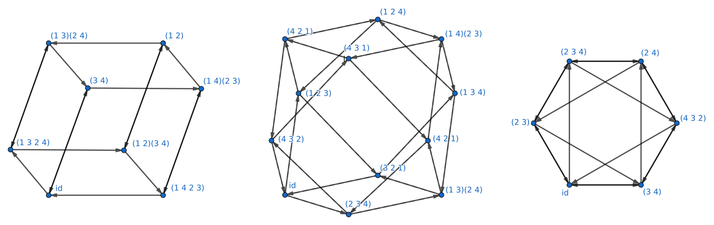
Middle: \{(1 ~ 2 ~ 3), (2 ~ 3 ~ 4)\}, cuboctahedral graph
Right: \{(2 ~ 3), (3 ~ 4), (2 ~ 3 ~ 4)\}, octahedral graph
Generating sets obtained from the previous MathWorld article.
Owing to the way in which they are defined, Cayley graphs have a few useful properties as graphs. At every vertex, we have as many outward edges as we do generators in the generating set, so the outward (and in fact, inward) degree of each vertex is the same. In other words, it is a regular graph. More than that, it is vertex-transitive, since labelling a single vertex’s outward edges will label that of the entire graph.
In general, the Cayley graph is a directed graph. However, if for every member of the generating set, we also include its inverse, every directed edge will be matched by an edge in the opposite direction, and the Cayley graph may be considered undirected.
Graphs to Graphs
All 2-cycles are their own inverse, so generating sets which include only them produce undirected Cayley graphs. Since this kind of generating set can itself be thought of as a graph, we may consider an operation on graphs that maps a swap diagram to its Cayley graph.
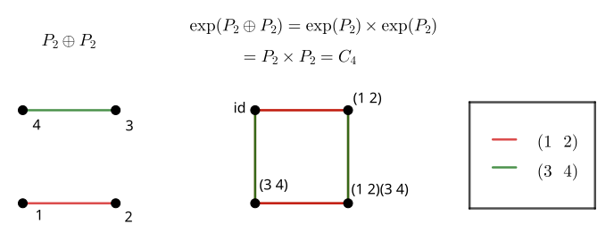
It seems to be the case that \exp( A \oplus B ) = \exp( A ) \times \exp( B ), where \oplus signifies the disjoint uinion and \times signifies the Cartesian (box) product of graphs2. Unlike γ from the previous post, both the input and output of this operation are graphs. Because of this and the sum/product relationship, I’ve taken to calling this operation the “graph exponential”3.
This operation is my own invention, so I am unsure whether or not it constitutes anything useful. In fact, the possible graphs grow so rapidly that computing anything about the exponential of order 8 graphs starts to overwhelm a single computer. It is, however, interesting, as I will hopefully be able to convince.
A random graph will not generally correspond to an interesting generating set, and therefore, will also generally have an uninteresting exponential graph. Hence, I will continue with the examples used previously: paths, stars, and complete graphs. They are among the simplest graphs one can consider, and as we will see shortly, have exponentials which appear to have natural correspondences to other graph families.
Some Small Exponential Graphs
Because of the difficulty in determining graph isomorphism, it is challenging for a computer to find a graph in an encyclopedia. Computers think of graphs as a list of vertices and their outward edges, but this implementation faces inherent labelling issues. These persist even if the graph is described as a list of (un)ordered pairs, an adjacency matrix, or an incidence matrix, the latter two of which have very large memory footprints4.
However, as visual objects, humans can compare graphs fairly easily – the name means “drawing” after all. Exponentials of order 3 and order 4 graphs are neither so small as to be uninteresting nor so big as to be unparsable by humans.
Order 3
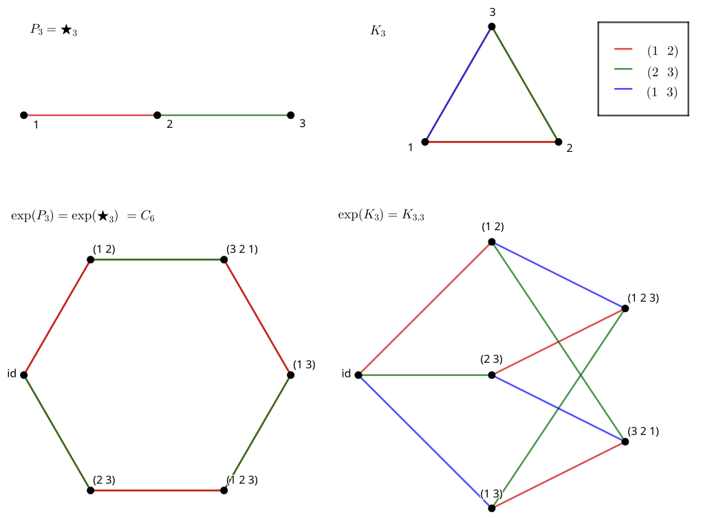
At this stage, we only really have two graphs to consider, since P_3 = \bigstar_3. Immediately, one can see that \exp( P_3 ) = \exp( \bigstar_3 ) = C_6, the 6-cycle graph (or hexagonal graph). It is also apparent that \exp( K_3 ) is the utility graph, K_{3,3}.
Note that the red element commutes with the green and blue ones. This produces two types of squares in the exponential graph. Meanwhile, the green and blue elements have an order 3 product, and produce the hexagon.
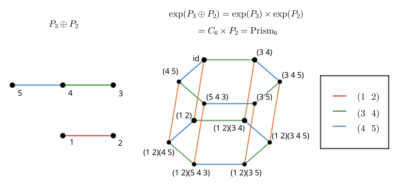
Here, we can again demonstrate the sum rule of the graph exponential with \exp( P_3 \oplus P_2 ). Simplifying, since we know \exp( P_3 ) = C_6, the result is C_6 \times P_2 = \text{Prism}_6, the hexagonal prism graph.
Order 4 (and beyond)


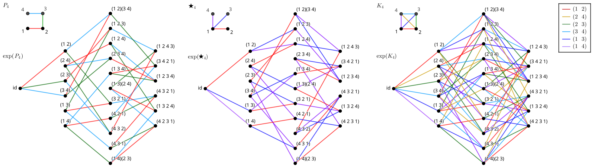
With some effort, \exp( P_4 ) can be imagined as a projection of a 3D object, the truncated octahedron. Because of its correspondence to a 3D solid, this graph is planar. Both the hexagon and this solid belong to a class of polytopes called permutohedra, which are figures that are also formed by permutations of the coordinate (1, 2, 3, …, n) in Euclidean space5. Technically, there is a distinction between the Cayley graphs and permutohedra since their labellings differ. Both have edges generated by swaps, but in the latter case, the connected vertices are expected to be separated by a certain distance. More information about the distinction can be found at this article on Wikimedia6.
Meanwhile, \exp( \bigstar_4 ) is more difficult to identify, at least without rearranging its vertices. It turns out to be isomorphic to the Nauru graph, a graph with many strange properties. Notably, whereas the graph isomorphic to the permutohedron is obviously a spherical polyhedron, the Nauru graph can be topologically embedded on a torus. The Nauru graph also belongs to the family of permutation star graphs PS_n (n = 4), which also includes the hexagonal graph (n = 3). The MathWorld article confirms some kind of correspondence, stating graphs of this form are generated by pairwise swaps.
My attempts at finding a graph isomorphic to \exp( K_4 ) have thus far ended in failure. It is certainly not isomorphic to K_{4,4}, since this graph has 8 vertices, as opposed to 24 in \exp( K_4 ).
Graph Invariants
While I have managed to identify the families to which some of these graphs belong, I am rather fond of computing (and conjecturing) sequences from objects. Not only is it much easier to consult something like the OEIS for these quantities, but after finding a matching sequence, there are ample articles to consult for more information. By linking to their respective entries, I hope you’ll consider reading more there.
Even though I have obtained these values empirically, I am certain that the sequences for \exp( P_n ) and \exp( \bigstar_n ) match the corresponding OEIS entries. I also have great confidence in the sequences I found for \exp( K_n ).
Edge Counts
Despite knowing how many vertices there are (n!, the order of the symmetric group), we don’t necessarily know how many edges there are.
| n | \#E(\exp( P_n )) | \#E(\exp( \bigstar_n )) | \#E(\exp( K_n )) |
|---|---|---|---|
| 3 | 6 | 6 | 9 |
| 4 | 36 | 36 | 72 |
| 5 | 240 | 240 | 600 |
| 6 | 1800 | 1800 | 5400 |
| 7 | 15120 | 15120 | 52920 |
| Sequence | Second column of Lah numbers OEIS A001286 |
Same as previous | OEIS 001809 |
| Rule | L(n,2) = n!{(n-1)(n-2) \over 4} | n!{n(n-1) \over 4} |
Radius and Distance Classes
The radius of a graph is the smallest possible distance which separates two maximally-separated vertices. Due to vertex transitivity, the greatest distance between two vertices is the same for every vertex.
| n | r(\exp( P_n )) | r(\exp( \bigstar_n )) | r(\exp( K_n )) |
|---|---|---|---|
| 3 | 4 | 4 | 3 |
| 4 | 7 | 5 | 4 |
| 5 | 11 | 7 | 5 |
| 6 | 16 | 8 | 6 |
| 7 | 22 | 10 | 7 |
| Sequence | Triangular numbers OEIS A000217 |
Integers not congruent to 2 (mod 3) OEIS A032766 |
n - 1 |
| Rule | \Delta_{n-1} = {n(n-1) \over 2} | \lfloor {n-1 \over 2} \rfloor + n -\ 1 |
These quantities are somewhat reductive. If a vertex is distinguished, the remaining vertices may be partitioned into classes by their distance from it. Including the vertex itself (which is distance 0 away), there will be r + 1 such classes, where r is the radius. These classes are the same for every vertex due to transitivity.
In the case of these graphs, they are a partition of n!.
| n | \text{dists}(\exp( P_n )) | \text{dists}(\exp( \bigstar_n )) | \text{dists}(\exp( K_n )) |
|---|---|---|---|
| 3 | [1, 2, 2, 1] | [1, 2, 2, 1] | [1, 3, 2] |
| 4 | [1, 3, 5, 6, 5, 3, 1] | [1, 3, 6, 9, 5] | [1, 6, 11, 6] |
| 5 | [1, 4, 9, 15, 20, 22, 20, 15, 9, 4, 1] | [1, 4, 12, 30, 44, 26, 3] | [1, 10, 35, 50, 24] |
| 6 | [1, 5, 14, 29, 49, 71, 90, 101 101, 90, 71, 49, 29, 14, 5, 1] |
[1, 5, 20, 70, 170, 250, 169, 35] | [1, 15, 85, 225, 274, 120] |
| 7 | [1, 6, 20, 49, 98, 169, 259, 359, 455, 531, 573 573, 531, 455, 359, 259, 169, 98, 49, 20, 6, 1] |
[1, 6, 30, 135, 460, 1110, 1689, 1254, 340, 15] | [1, 21, 175, 735, 1624, 1764, 720] |
| Sequence | Mahonian numbers OEIS A008302 |
Whitney numbers of the second kind (star poset) OEIS A007799 |
Stirling numbers of the first kind OEIS A132393 |
I am certain that the appearance of the Stirling numbers here is legitimate, since these numbers count the number of permutations of n objects with k disjoint cycles. Obviously, the identity element is distance 1 from all 2-cycles since they are all in the generating set; likewise, all 3-cycles are distance 2 from the identity (but distance 1 from the 2-cycles), and so on until the entire graph has been mapped. The shapes induced by these classes were used to create the diagrams of \exp( K_3 ) and \exp( K_4 ) above.
Spectrum
The eigenvalues of the adjacency matrix of a graph can be interesting and sometimes help in identifying a graph. Unfortunately, eigenvalues are not necessarily integers, and therefore not easily found in the OEIS (though they are always real for graphs).
| n | \text{Spec}(\exp( P_n )) | \text{Spec}(\exp( \bigstar_n ) | \text{Spec}(\exp( K_n )) |
|---|---|---|---|
| 3 | \begin{gather*}(\pm1)^{2\phantom{0}} \\ (\pm2)^{1\phantom{0}}\end{gather*} | \begin{gather*}(\pm1)^{2\phantom{0}} \\ (\pm2)^{1\phantom{0}}\end{gather*} | \begin{gather*}(0)^{4\phantom{0}} \\ (\pm3)^{1\phantom{0}}\end{gather*} |
| 4 | \begin{gather*}(\pm1)^{3} (\pm3)^{1} \\ \left(x^{2} - 3\right)^{2} \\ \left(x^{2} + 2 x - 1\right)^{3} \\ \left(x^{2} - 2 x - 1\right)^{3} \\ \left(x^{2} + 2 x - 1\right)^{3} \\ \left(x^{2} - 2 x - 1\right)^{3}\end{gather*} | \begin{gather*}(0)^{4\phantom{0}} \\ (\pm1)^{3\phantom{0}} \\ (\pm2)^{6\phantom{0}} \\ (\pm3)^{1\phantom{0}}\end{gather*} | \begin{gather*}(0)^{4\phantom{0}} \\ (\pm2)^{9\phantom{0}} \\ (\pm6)^{1\phantom{0}}\end{gather*} |
| 5 | \begin{gather*}(0)^{12} (\pm1)^{6} (\pm4)^{1} \\ \left(x^{2} - 5\right)^{6} \\ \left(x^{2} - 5 x + 5\right)^{4} \\ \left(x^{2} + 5 x + 5\right)^{4} \\ \left(x^{2} - 3 x + 1\right)^{4} \\ \left(x^{2} + 3 x + 1\right)^{4} \\ \left(x^{2} + 2 x - 1\right)^{5} \\ \left(x^{2} - 2 x - 1\right)^{5} \\ \left(x^{3} + 2 x^{2} - 5 x - 4\right)^{5} \\ \left(x^{3} - 2 x^{2} - 5 x + 4\right)^{5}\end{gather*} | \begin{gather*}(0)^{30\phantom{00}} \\ (\pm1)^{4\phantom{00}} \\ (\pm2)^{28\phantom{00}} \\ (\pm3)^{12\phantom{00}} \\ (\pm4)^{1\phantom{00}}\end{gather*} | \begin{gather*}(0)^{36\phantom{00}} \\ (\pm2)^{25\phantom{00}} \\ (\pm5)^{16\phantom{00}} \\ (\pm10)^{1\phantom{00}}\end{gather*} |
| 6 | \begin{gather*}(0)^{20} (\pm1)^{25} (\pm2)^{15}\\(\pm3)^{5} (\pm4)^{5} (\pm5)^{1} \\ \left(x^{2} - 3\right)^{20}\end{gather*}Not shown: 558 other roots | \begin{gather*}(0)^{168\phantom{000}} \\ (\pm1)^{30\phantom{000}} \\ (\pm2)^{120\phantom{000}} \\ (\pm3)^{105\phantom{000}} \\ (\pm4)^{20\phantom{000}} \\ (\pm5)^{1\phantom{000}}\end{gather*} | \begin{gather*}(0)^{256\phantom{000}} \\ (\pm3)^{125\phantom{000}} \\ (\pm5)^{81\phantom{000}} \\ (\pm9)^{25\phantom{000}} \\ (\pm15)^{1\phantom{000}}\end{gather*} |
| 7 | \begin{gather*}(0)^{35\phantom{00}} \\ (\pm1)^{20\phantom{00}} \\ (\pm2)^{45\phantom{00}} \\ (\pm6)^{1\phantom{00}}\end{gather*}Not shown: 4873 other roots | \begin{gather*}(0)^{840\phantom{000}} \\ (\pm1)^{468\phantom{000}} \\ (\pm2)^{495\phantom{000}} \\ (\pm3)^{830\phantom{000}} \\ (\pm4)^{276\phantom{000}} \\ (\pm5)^{30\phantom{000}} \\ (\pm6)^{1\phantom{000}}\end{gather*} | \begin{gather*}(0)^{400\phantom{0000}} \\ (\pm1)^{441\phantom{0000}} \\ (\pm3)^{1225\phantom{0000}} \\ (\pm6)^{196\phantom{0000}} \\ (\pm7)^{225\phantom{0000}} \\ (\pm9)^{196\phantom{0000}} \\ (\pm14)^{36\phantom{0000}} \\ (\pm21)^{1\phantom{0000}}\end{gather*} |
| 8 | Not shown: all 40320 roots | \begin{gather*}(0)^{3960\phantom{0000}} \\ (\pm1)^{5691\phantom{0000}} \\ (\pm2)^{2198\phantom{0000}} \\ (\pm3)^{6321\phantom{0000}} \\ (\pm4)^{3332\phantom{0000}} \\ (\pm5)^{595\phantom{0000}} \\ (\pm6)^{42\phantom{0000}} \\ (\pm7)^{1\phantom{0000}}\end{gather*} | \begin{gather*}(0)^{9864\phantom{0000}} \\ (\pm2)^{3136\phantom{0000}} \\ (\pm4)^{6125\phantom{0000}} \\ (\pm7)^{4096\phantom{0000}} \\ (\pm8)^{196\phantom{0000}} \\ (\pm10)^{784\phantom{0000}} \\ (\pm12)^{441\phantom{0000}} \\ (\pm20)^{49\phantom{0000}} \\ (\pm28)^{1\phantom{0000}}\end{gather*} |
From what I have been able to identify, the spectrum of an exponential graph is symmetric about 0, by which I mean that the characteristic polynomial is even. This has been the case for all graphs I have tried testing, even outside these graph families.
Since all eigenvalues of \exp( \bigstar_n ) calculated are integers, it appears they are integral graphs, a fact of which I am reasonably sure because of the aforementioned correspondence to permutation star graphs. Additionally, the eigenvalues are very conveniently the integers up to n-1 and down to -n+1. Unfortunately, despite the ease of reading the eigenvalues themselves, there isn’t an OEIS entry for the multiplicities. I was able to identify the multiplicity of the 0 eigenvalue with OEIS A217213, which counts orderings on Dyck paths. If this is truly the sequence being generated, it means there is a 1:1 correspondence between these orderings and a basis of the nullspace of the adjacency matrix.
It seems to be the case that \exp( K_n ) are also integral graphs. Perplexingly, the multiplicities for each of the eigenvalues appear to mostly be perfect powers. This is the case until n = 8, which ruins the pattern because neither of 9864 = 2^3 \cdot 3^2 \cdot 137 or 6125 = 5^3 \cdot 7^2 are perfect powers. I find both this7 and the fact that such a large prime appears among the factorization of the former rather creepy since all other primes which appear here are small – 2, 3, 5, and 7.
Notes about Spectral Computation
For n = 3 through 6, exactly computing the spectrum (or more accurately, the characteristic polynomial) is possible, although it takes upwards of 10 minutes for n = 6 on my machine using sympy. The spectra of n = 7, 8 are marked with an asterisk because they were computed numerically, which still took nearly 8 hours in the case of the latter. In fact, these graphs grow so quickly that it becomes nearly impossible to compute the spectrum without an explicit formula.
For n = 8, even storing the adjacency matrix in memory is a problem. Assuming the use of single-precision floating point, this behemoth of a matrix is (8!)^2 \cdot 4 \text{ bytes} = 6.5\text{GB}. This doesn’t even factor in additional space requirements for eigenvalue algorithms, and is the reason I certainly won’t be attempting to compute the spectrum for n = 9.
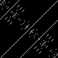
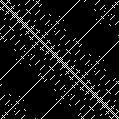
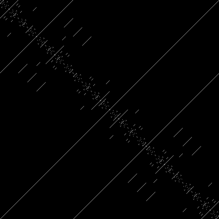
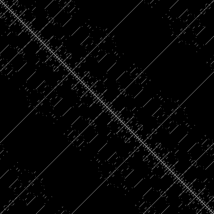
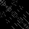
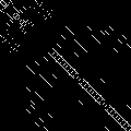
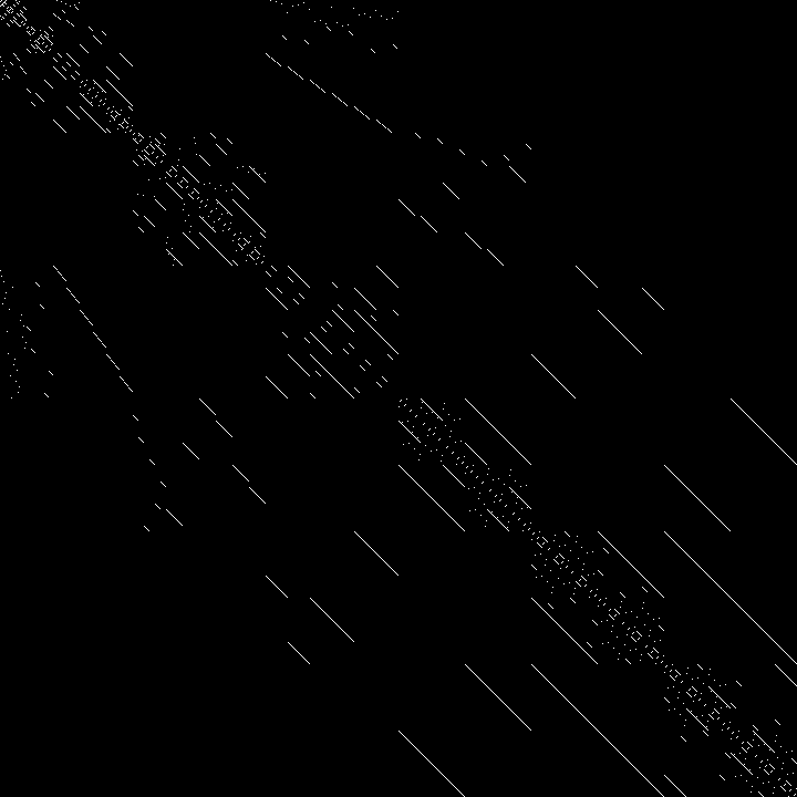
Gallery of Adjacency Matrices
The patterns in adjacency matrices depend on an enumeration of S_n so that the vertices can be labelled from 1 to n!. While this is a fascinating topic unto itself, this post is already long enough, and I feel comfortable with just sharing the pictures.
Plain Changes
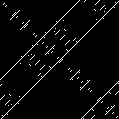
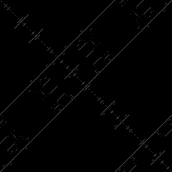
Heap’s Algorithm
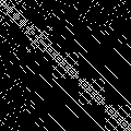
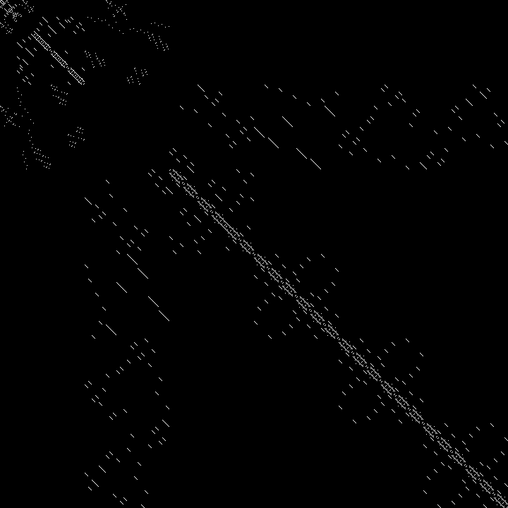
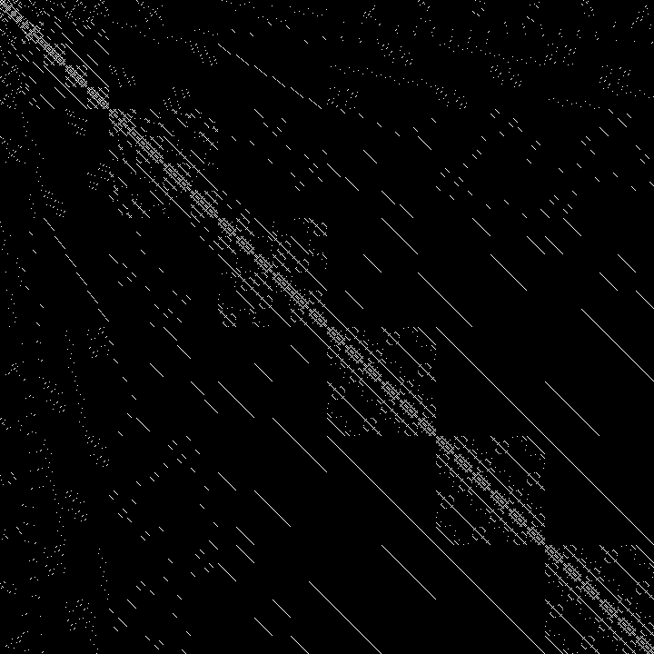
Note: GHC’s Data.List.permutations is slightly different from Heap’s algorithm as displayed on Wikipedia
Closing
As previously stated, I am only mostly sure of the validity of the exponential law for graphs. It seems too good to be true, but testing it directly on some graphs by comparing the spectra of the exponential of the sum against the product of the exponentials shows that they are at least cospectral. Try it yourself, preferably with a better tool than the ones I made in Haskell.
From the articles I was able to find, permutation star graphs have applications to parallel computing, which is somewhat ironic considering how little care I had for the topic when writing this article. If I needed ruthless efficiency, I probably could have used a library with GPU algorithms (or taken a stab at writing a shader myself). However, I was able to use this as a learning experience regarding mutable objects in Haskell. With only immutable objects (and enough garbage to create an island in the Pacific), I was running out of memory even with 16GB of RAM and 16GB of swap. Introducing mutability not only brought improvements in space, but also a great deal of speedup, enough to make rendering adjacency matrix images of order 8 graphs just barely doable within a reasonable time span.
Said images are cursed. Remember, as raw bitmaps, these files are on the order of gigabytes big. On a much weaker computer than I used to render the images, merely opening my file explorer to the folder containing the folder containing the images caused its all-too-eager thumbnailer to run. This started consuming all of my system resources, crashed all of my browser’s tabs, distorted audio, and finally locked up the computer. Despite this, PNG is a wonderful format that is able to compress them down to just 4MB, which demonstrates just how sparse these matrices are.
Despite everything I was able to find about permutation star graphs and permutohedra, I was surprised that there is no information about the Cayley graphs generated by all 2-cycles (or at least information which is easy to find). This is especially disappointing considering the phantom pattern which gets destroyed by 137, and I would love to know more about why this happens in the first place.
Graph diagrams made with GeoGebra and NetworkX (GraphViz).
Additional Links
- Whitney Numbers of the Second Kind for the Star Poset ( Paper from ScienceDirect )
- This article includes a section about representing a list of generators as a graph, making me wonder if someone has tried defining this operation before
- Whitney Numbers (Josh Cooper’s Mathpages)
- The Many Faces of the Nauru Graph (Blogpost by David Eppstein)
Footnotes
The construction implies a labelling of edges by its generating set and a labelling of vertices by the generated elements. It is also common to describe an unlabelled graph as “Cayley” if it could be generated by this procedure.↩︎
Graphs have many product structures, such as the tensor product and strong product. The Cartesian product is (categorically) more natural when paired with disjoint unions.↩︎
Originally, I called this operation the “graph factorial”, since it involves permutations and the number of vertices in the resulting graph grows factorially.↩︎
I was able to locate a project named the Encyclopedia of Finite Graphs, but it is only able to build a database simple connected graphs which can be queried by invariants (and is outdated since it uses Python 2).↩︎
In fact, these figures are able to completely tessellate the n-1 dimensional subspace of \mathbb{R}^n where the coordinates sum to the n-1th triangular number. Note also that the previous graph in the sequence of \exp(P_n), the hexagonal graph, is visible in the truncated octahedron. This corresponds to the projection (x,y,z,w) \mapsto (x,y,z) over the coordinates of the permutohedra.↩︎
Actually, if one considers a right Cayley graph, where each generator is right-multiplied to the permutation at a node rather than left-multiplied, then a true correspondence is obtained, at least for order 4.↩︎
Some physicists are fond of 137 for its closeness to the reciprocal of the fine structure constant (a bit of mostly-harmless numerology).↩︎