A Game of Permutations, Part 3
Extending swap diagrams (with apologies to H.S.M. Coxeter).
This post assumes you have read the first post, which talks about swap diagrams and the symmetric group. The section about Cayley graphs from the second post will also be useful.
To summarize from the first post, a swap diagram is a graph where each vertex represents a list index and each edge represents the permutation which swaps the two entries. I singled out three graph families for their symmetry:
- Paths, which link adjacent swaps
- Stars, in which all swaps contain a distinguished index
- Complete graphs, which contain all possible swaps
Swap diagrams are ultimately limited by only being able to describe collections of 2-cycles. If we wanted to include higher-order elements, we’d require a weaker mathematical structure called a hypergraph. These are even more difficult to draw than simple graphs, much less understand.
Another way we are limited is in the kinds of groups which can be encoded. One can rather quickly notice that swap diagrams will only generate symmetric groups and direct products thereof. Also, while edges are members of a generating set, the vertices contain information which is ultimately irrelevant to the group.
Upgrading Diagrams
What if we forgot the roles of the vertices, allowed the edges to take their place? In other words, we want to make a graph where the vertices represent generators, rather than the edges.
Ideally, we’d still like to preserve some information about coincident edges. Graph-theoretically, we can elevate the role of the edges to that of the vertices by making a line graph. This operation produces a graph such that
- Every edge in the original graph becomes a vertex in the new graph
- Coincident edges in the new graph are connected by an edge in the new graph
- In other words, we convert adjacent edges to adjacent vertices.
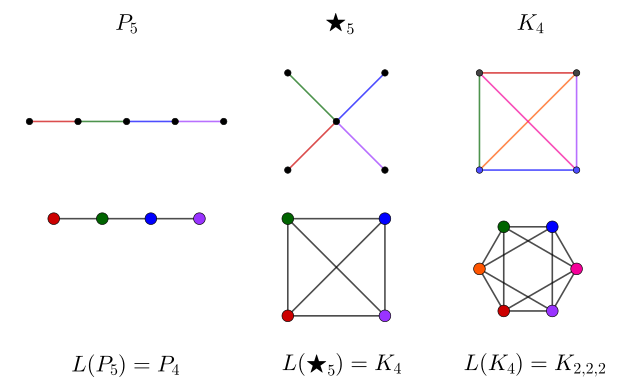
The line graph of a swap diagram results in a graph where the vertices are the 2-cycles. In a swap diagram, when two distinct 2-cycles share an index (vertex), their product has order 3. Thus, in the line graph, the edges mean that the product of the two vertices has order 3. Non-adjacent vertices still have a product with order 2, since they represent disjoint 2-cycles.
To push the group/graph correspondence the even further, we can impose a final restriction. Namely, a subgraph should represent a subgroup. Specifically, we want an induced subgraph (one where if two connected vertices are included, then so is the edge joining them) since this maintains the relationship between the generators. Unfortunately, this restriction disqualifies many of the line graphs of swap diagrams. At least our beloved paths are left untouched, since L(P_n) = P_{n-1}.
Coxeter Diagrams
As it turns out, these restrictions are significant and produce some very deep mathematical objects, known as Coxeter diagrams (named for the same Coxeter as in Goldberg-Coxeter). In this domain, the aforementioned rules about vertices and edges apply: each vertex corresponds to an order 2 element and each edge signifies that the product of two elements has order 3. Furthermore, disconnected vertices correspond to elements which commute with one another, just like disjoint 2-cycles. However, each vertex need not correspond to a single 2-cycle, and can instead be any element of order 2, i.e., a product of disjoint 2-cycles.

Source: Rgugliel, via Wikimedia Commons
Coxeter diagrams are frequently extended to enable describing higher-order products by labelling the edge1. For example, the product between (1 ~ 2)(3 ~ 4) and (2 ~ 3) has order 4. A diagram for these elements would therefore include two vertices connected with an edge labelled “4”, corresponding to B_2.
How Big and What Shape?
We already know how big the group a swap diagram generates. Each connected component with n vertices generates the group S_n. They combine via the direct product to give a group of order
\left | \prod_i S_{n_i} \right | = \prod_i | S_{n_i} | = \prod_i n_i!
Removing an edge from a swap diagram has the potential to make the graph disconnected. In this case, the graph is split into two parts, which map to S_m and S_n. This tells us that S_m \times S_n embeds in S_{m + n}.
The subgroup restriction makes Coxeter diagrams a lot more sensitive to changes. We at least know that if we remove a vertex, the resulting diagram is a subgroup of the whole diagram. What we need is some way to measure the effect this has on the rest of the group.
Coxeter-Todd Algorithm
This is exactly what the Coxeter-Todd algorithm does. It more-or-less generalizes the procedure for creating Cayley graphs. Using the vertices of the Coxeter diagram as generators2, we convert products between them to paths in a graph.
Let’s apply the algorithm to the diagram A_3. First, we need to label our generators as a, b, and c. Then, we select a select a generator to remove and create a graph according to the following steps:
1. Initialization
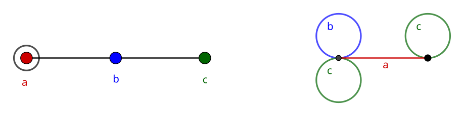
In a Cayley graph, we start out with a single vertex representing the identity. Here, the first vertex instead corresponds to the subgroup generated by all other generators.
For each generator other than the one being removed, we attach loops to the vertex. This is because the subgroup is closed – when we multiply the set of all elements of the subgroup by any of its elements, it doesn’t change the set. In other words, hH = H, h \in H.
For the remaining generator, we draw an edge connecting to a new vertex, which represents a new set of elements. This is a coset of the subgroup – that is, each vertex we make in this new graph corresponds to a disjoint partition of elements of the whole group.

Right: the first step of generating a graph from removing generator a. The (group generated by the) bc subdiagram is represented by the vertex with the b and c loops.
Note that all loops and edges we draw will be undirected, since all generators have order 2. Performing the same operation twice just takes us back to where we started.
2. Loop Transference
At the new vertex, we transfer over every loop whose label is not connected to the label of the edge. This is due to the rule stating that non-adjacent generators commute. In other words, their product has order 2. For our graph, this can be seen for acac = a^2 c^2 = \text{id} = (ac)^2, and means after following labels acac, we end up at the same vertex we started at.
3. Extension, Branching, and Rejoining
At the new vertex, we still need an edge labelled b, but it cannot be a loop. Adjacent generators have a product whose order is the label (n) of the edge connecting them (defaulting to 3 for unlabelled ones). This means we need to form a path alternating between the two generators, such that following it would loop back to the vertex we started at. That is,
(ab)^n = \stackrel{n \text{ times}}{\overbrace{(ab)(ab) ... (ab)(ab)}} = \text{id}
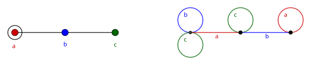
If the Coxeter diagram branches, then so does the generated graph. The labels of each pair of branching edges have a product with a known order, so following a path alternating between two of them must return to the same vertex. Since it alternates between the two labels n times, this ends up producing even-sided polygons in our generated graph. Commuting vertices form either a square or a pair of loops connected by an edge. The latter is actually a special case of the former, which can be seen by matching a pair of opposite edges.

Bottom: two adjacent vertices form a hexagon
4. Finalization
If we ensure at each new vertex that we can follow a valid path for every pair of generators, then this process will either terminate or continue indefinitely with a repeating pattern. A quick sanity check on the resulting graph is to add the number of loops and edges at a vertex. The sum should be the number of generators.
As stated earlier, each vertex in the graph corresponds to a coset of the group under the subgroup being considered. The number of cosets is the index of the subgroup, the quantity we were after the whole time. In this case, the index of the three-vertex diagram (A_3) on the two-vertex diagram (A_2, the same diagram without a) is 4.
Results
We can remove vertices one-by-one until we eventually reduce the graph to a single vertex, which we know has order 2. Multiplying all of the indices at each stage together gives us the order of the group we are after.
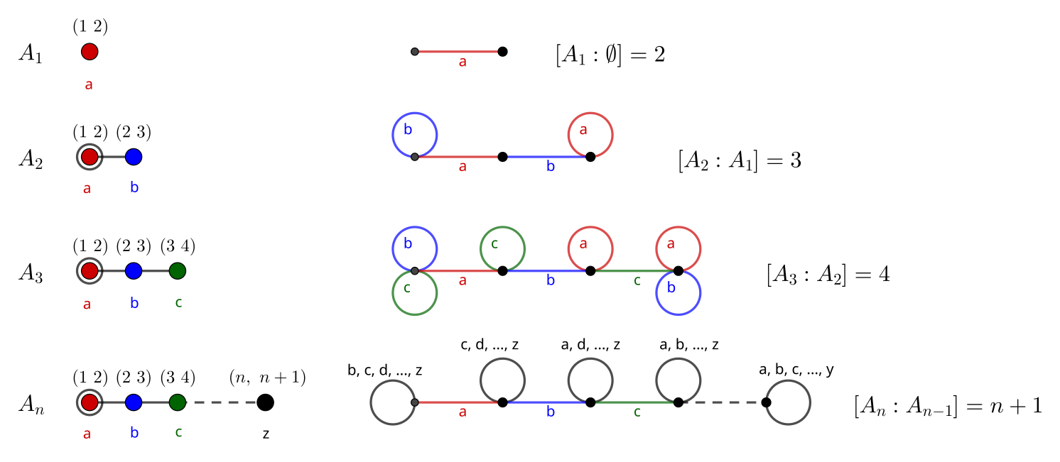
Permutations shown above vertices which give a permutation group embedding.
It is readily shown that the group generated by A_3 has order 4 \cdot 3 \cdot 2 = 24, which coincides with the order of S_4.
We can assign a permutation to each of our generators, so long as the edge condition as it relates to their product is obeyed. In the diagrams above, (1 ~ 2) and (2 ~ 3) have a product of order 3, but (1 ~ 2) and (3 ~ 4) have a product of order 2, since the cycles (and in the diagram, the vertices) are disjoint. This argument generalizes nicely to higher A_n.
Other Diagrams for A_3
A path is hardly the most interesting diagram. However, there are yet more graphs which can be produced from A_3.
Starting in the Middle
Selecting either endpoint of the diagram (generator a or c) will generate the same graph as shown above. This is easy to see if you read the generated graph right-to-left rather than left-to-right. However, the center point b has two neighbors. If we try generating a graph by removing this generator, our graph branches.
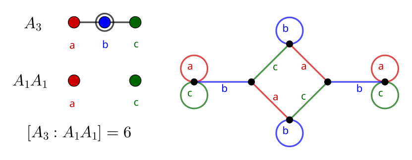
The index of 6 given by this graph is correct, since the remaining diagram A_1 A_1 has an order of 2 \cdot 2 = 4. This group is isomorphic to the Klein four-group, so this diagram shows that it occurs within S_4.
Removing Multiple Vertices
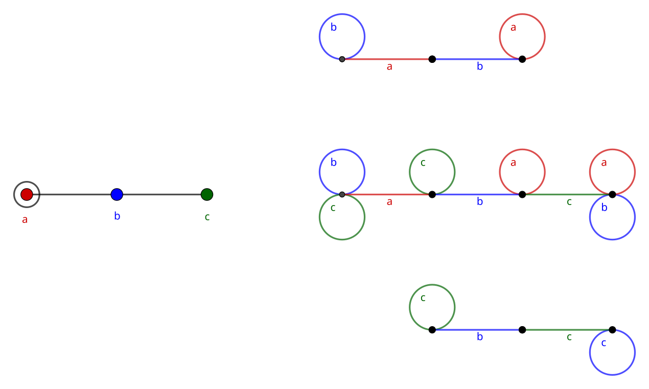
We can remove more than one generator from the Coxeter diagram at once, as long as we follow all the rules. Instead, the initial vertex in the new graph branches immediately and has fewer loops. For example, removing two generators from A_3 produces a figure with squares and hexagons:
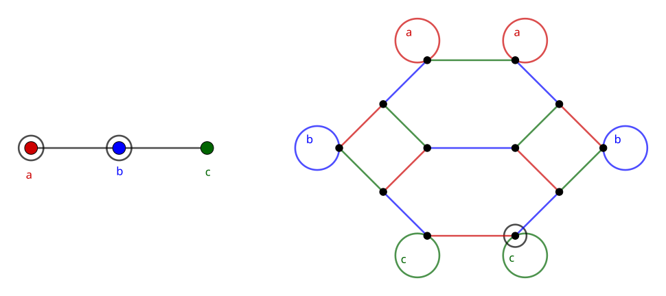
For the circled generators a and b, the diagram starts from the circled vertex on the right (or its identical neighbor).
If b and c were removed instead, the diagram would start from the similar vertices with a loops at the top of the graph.
If a and c were removed, the diagram would start from either the leftmost or rightmost vertex, which both have a b loop.
A figure composed of squares and hexagons should be familiar from the previous post. The truncated octahedron also contains only squares and hexagons and is generated by S_4. In fact, the figure above is the truncated octahedron folded in half. It is folded in “half” specifically because the single remaining vertex in the Coxeter diagram has order 2. Consequently, the number of vertices in the graph must be half that of the whole group (or complete permutahedron).
If we remove both generators in A_2, we end up with a hexagon.
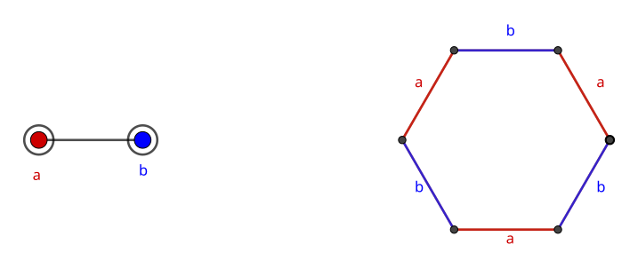
Also from the previous post, we know this to be the Cayley graph for S_3 generated by a pair of swaps. In this way, the Cayley graph can be thought of as a sort of “limiting” graph of the Coxeter diagram, where each coset contains only a single element.
The Traditional Explanation
I must now admit that that I have not given anywhere near the whole explanation of Coxeter diagrams, and have only succeeded in leading us down the proverbial algebraic rabbit hole.
Coxeter diagrams also come equipped with a standard geometric interpretation. The “order 2 elements” we discussed previously are replaced with mirrors, and the edge labels are the angle between mirrors, interpreted as half of the central angle of a regular n-gon (triangle: 60°, square: 45°, …).


Source: Tomuren, via Wikimedia Commons
The image above is composed of the mirrors specified by A_2. One of the generators is the red reflection and the other is the the green reflection. It is clear that alternating between red and green three times will take one back to where they started, just like the algebra tells us.
All of the plane ends up assigned to one of the domains. Note also that points along mirrors which are equidistant from the center form a hexagon made up of six equilateral triangles, one in each domain.
Struggles in 3D
A_3 has an additional vertex and edge. This means that an additional mirror needs to be placed in along every preexisting reflection. We end up reflecting into another dimension, and our domains shoot out into 3D space. It is easier to imagine the additional domains by rotating two of the axes around each other, so that the pairs will join together into equilateral triangular “cones”.
In 2D, equidistant points form a hexagon; in 3D, the points instead form a cuboctahedron. Connecting the triangular faces of the cuboctahedron to the origin gives a family of eight tetrahedra meeting at a point. At this point the reflections become clearer, since certain reflections do the same thing as in the plane above, while others will “double” a tetrahedron.


Personally, I think the geometric way of thinking becomes is difficult even in 3D. Every axis describes a separate rotation, which is simple enough. But we’re trying to create infinite cones of symmetry domains in 3D space, and we can only try to interact with this using a 2D screen. We’re running out of room before even getting to 4D space, where the visualization problems are even worse. Also, while the angle between two mirrors is 60°, it’s easy to slip into thinking about the dihedral angle between two faces (domains) of the cones, which is not 60°.
Closing
When I initially wrote the article about swap diagrams (a name I hadn’t given them at the time) I had no idea about how closely it related to something else which I was having trouble understanding. Now knowing better, I split the article and pushed the basics a little harder. I find this closeness between swap diagrams and Coxeter diagrams interesting. At the cost of simplicity, the latter enables the ability to encode higher-order cycles and give rise to exceptional mathematical objects.
It was difficult for me to find information documenting how to understand the algebraic perspective. It also bears mentioning that I know very little about Lie theory, another field of math where Coxeter diagrams turn up. When I finally found a group theory video by Professor Richard Borcherds, I was dismayed that there seems to be even less material online which depicts the coset graphs. I have written an appendix cataloguing some graphs that appear when applying the Coxeter-Todd algorithm, since I believe they are interesting in their own right.
Images from Wikimedia belong to their respective owners. All other diagrams created with GeoGebra.