from itertools import count, chain, islice, takewhile
import numpy as np

def fibs():
    i = 1
    j = 1
    while True:
        yield i
        t = i + j
        j = i
        i = t

def zeck(n: int) -> list[int]:
    fibs_ = list(takewhile(lambda x: x <= n, fibs()))[::-1]
    ret = []

    for i in fibs_:
        digit, n = divmod(n, i)
        ret.append(digit)

    return ret or [0]

def unzeck(ns: list[int]) -> int:
    return sum(map(lambda x, y: x * y, reversed(ns), fibs()))

def zeck_times(x: int, y: int) -> int:
return unzeck(np.convolve(zeck(x), zeck(y), "full"))Polynomial Counting 5: Pentamerous multiplication
algebra
python
Arithmetic in non-geometric integral systems and surprisingly regular errors therein.
This post assumes you have read the first, which introduces generalized polynomial counting.
One layer up from counting is arithmetic. We’ve done a little arithmetic using irrational expansions in pursuit of counting, but maybe we should investigate it a bit.
Arithmetical Algorithms
Addition is a fairly simple process for positional systems: align the place values, add each term together, then apply the carry as many times as possible. Without a carry rule, this can be approached formally by treating the place values as a sequence b_n and gathering terms:
\begin{gather*} \phantom{+~} \overset{b_2}{1} \overset{b_1}{2} \overset{b_0}{3} & \phantom{+~} 1b_2 + 2b_1 + 3b_0 \\ \underline{ +\ \smash{ \overset{\phantom{b_0}}4 \overset{\phantom{b_0}}5 \overset{\phantom{b_0}}6 } \vphantom, } & \underline{ +\ 4b_2 + 5b_1 + 6b_0 \vphantom, } \\ \phantom{+~} \smash{ \overset{\phantom{b_0}}5 \overset{\phantom{b_0}}7 \overset{\phantom{b_0}}9 } & \phantom{+~} 5b_2 + 7b_1 + 9b_0 \end{gather*}
Multiplication is somewhat trickier. Its validity follows from the interpretation of an expansion as a polynomial. Polynomial multiplication itself is equivalent to discrete convolution.
\begin{align*} &\begin{matrix} \phantom{\cdot~} 111_x \\ \underline{\cdot\ \phantom{1}21_x\vphantom,} \\ \phantom{\cdot \ 0} 111_{\phantom{x}} \\ \underline{\phantom{\cdot\ } 2220_{\phantom{x}} \vphantom,} \\ \phantom{\cdot\ } 2331_{\phantom{x}} \end{matrix} &\qquad& \begin{gather*} (x^2 + x + 1)(2x + 1) \\ \\ = \phantom{2x^3 + } \phantom{2}x^2 + \phantom{2}x + 1 \\ + \phantom{.} 2x^3 + 2x^2 + 2x \phantom{+ 1}\\ = 2x^3 + 3x^2 + 3x + 1 \end{gather*} &\qquad& \begin{gather*} [1,1,1] * [2,1] \\ \begin{matrix} \textcolor{blue}0 &\textcolor{red}1 & \textcolor{red}1 & \textcolor{red}1 & \textcolor{blue}0 &\\ & & &1 & 2 & =~1\\ & & 1 & 2 & &=~3\\ & 1 & 2 & & &=~3\\ 1 & 2 & & & & =~2 \end{matrix} \end{gather*} \end{align*}
The left equation shows familiar multiplication, the middle equation is the same product when expressed as polynomials, and the right equation shows this product obtained by convolution. Note that [2, 1], the second argument, is reversed when performing the convolution.
Without carrying, multiplication and addition are base-agnostic. When doing arithmetic in a particular base, we should obtain the same result even if we perform the same operations in another base.
\begin{array}{c} 18_{10} \cdot 5_{10} = 10010_2 \cdot 101_2 \\ \hline \\ \begin{gather*} & \begin{matrix} \phantom{\cdot~} 18_{10} \\ \underline{\cdot\ \phantom{1}5_{10}\vphantom,} \\ \phantom{\cdot~}90_{10} \\ \\ =~1011010_2 \end{matrix} && \begin{matrix} [1,0,0,1,0] * [1,0,1] \\ \\ \begin{matrix} \textcolor{blue}0 & \textcolor{blue}0 &\textcolor{red}1 & \textcolor{red}0 & \textcolor{red}0 & \textcolor{red}1 & \textcolor{red}0 & \textcolor{blue}0 & \textcolor{blue}0 &\\ & & & & & &1 & 0 & 1 & =~0\\ & & & & &1 & 0 & 1 & & =~1\\ & & & &1 & 0 & 1 & & & =~0\\ & & &1 & 0 & 1 & & & & =~1\\ & &1 & 0 & 1 & & & & & =~1\\ & 1 & 0 & 1 & & & & & & =~0\\ 1 & 0 & 1 & & & & & & & =~1\\ \end{matrix} \end{matrix} \end{gather*} \end{array}
This shows that regardless of whether we multiply eighteen and five together in base ten or two, we’ll get the same string of digits if afterward everything is rendered in the same base. Fortunately in this instance, we don’t have to worry about any carries in the result.
Two Times Tables
The strings “10010” and “101” do not contain adjacent “1”s, so they can also be interpreted as Zeckendorf expansions (of ten and four, respectively). This destroys their correspondence to polynomials, so their product by convolution, as a Zeckendorf expansion (when returned to canonical form) is not the product of ten and four.
\begin{gather*} [1,0,0,1,0] * [1,0,1] = 1011010 \\ 10\textcolor{red}{11}010_{\text{Zeck}} = 1\textcolor{red}{1}00010_{\text{Zeck}} = \textcolor{blue}{11}00010_{\text{Zeck}} = \textcolor{blue}{1}0000010_{\text{Zeck}} = 36_{10} \\ \text{Zeck}(10_{10}) * \text{Zeck}(4_{10}) = 36_{10} \neq 40_{10} = 10_{10} \cdot 4_{10} \end{gather*}
We can express this operation for general integers x and y as
x \odot_\text{Zeck} y = \text{Unzeck}(\text{Zeck}(x) * \text{Zeck}(y))
where “Zeck” expands an integer into its Zeckendorf expansion and “Unzeck” signifies the process of re-interpreting the string as an integer. We can do this because for every integer, a canonical expansion exists. Further, since this operation is defined via convolution (which is commutative), it is also commutative.
We can then build a times table by experimentally multiplying. The expansions for zero and one are invariably the strings “0” (or the empty string!) and “1”. When a sequence has length one, convolution degenerates to term-by-term multiplication. Thus, convolution by “0” produces a sequence of “0”s, and convolution by “1” produces the same sequence.
Ignoring those rows, the table is:
Code
from IPython.display import Markdown
from tabulate import tabulate

Markdown(tabulate(
    [[zeck_times(i, j) for i in range(1, 10)] for j in range(2, 10)],
    headers=["$\\odot_\\text{Zeck}$", *range(2, 10)]
))| \odot_\text{Zeck} | 2 | 3 | 4 | 5 | 6 | 7 | 8 | 9 |
|---|---|---|---|---|---|---|---|---|
| 2 | 3 | 5 | 7 | 8 | 10 | 11 | 13 | 15 |
| 3 | 5 | 8 | 11 | 13 | 16 | 18 | 21 | 24 |
| 4 | 7 | 11 | 15 | 18 | 22 | 25 | 29 | 33 |
| 5 | 8 | 13 | 18 | 21 | 26 | 29 | 34 | 39 |
| 6 | 10 | 16 | 22 | 26 | 32 | 36 | 42 | 48 |
| 7 | 11 | 18 | 25 | 29 | 36 | 40 | 47 | 54 |
| 8 | 13 | 21 | 29 | 34 | 42 | 47 | 55 | 63 |
| 9 | 15 | 24 | 33 | 39 | 48 | 54 | 63 | 72 |
This resembles a sequence in the OEIS (A101646), where it mentions the defining operation is sometimes called the “arroba” product.
Correcting for Errors
The difference between the actual product and the false product can be interpreted as an error endemic to Zeckendorf expansions. If assigned to the symbol \oplus_\text{Zeck}, then the normal product can be recovered as mn = m \odot_\text{Zeck} n + m \oplus_\text{Zeck} n.
We can then tabulate these errors just like we did our “products”:
Code
zeck_error = lambda x, y: x*y - zeck_times(x, y)

Markdown(tabulate(
    [[j] + [zeck_error(i, j) for i in range(2, 10)] for j in range(2, 10)],
    headers=["$\\oplus_\\text{Zeck}$", *range(2, 10)]
))| \oplus_\text{Zeck} | 2 | 3 | 4 | 5 | 6 | 7 | 8 | 9 |
|---|---|---|---|---|---|---|---|---|
| 2 | 1 | 1 | 1 | 2 | 2 | 3 | 3 | 3 |
| 3 | 1 | 1 | 1 | 2 | 2 | 3 | 3 | 3 |
| 4 | 1 | 1 | 1 | 2 | 2 | 3 | 3 | 3 |
| 5 | 2 | 2 | 2 | 4 | 4 | 6 | 6 | 6 |
| 6 | 2 | 2 | 2 | 4 | 4 | 6 | 6 | 6 |
| 7 | 3 | 3 | 3 | 6 | 6 | 9 | 9 | 9 |
| 8 | 3 | 3 | 3 | 6 | 6 | 9 | 9 | 9 |
| 9 | 3 | 3 | 3 | 6 | 6 | 9 | 9 | 9 |
Notice that the errors seem to be grouped together in rectangular blocks. Because this operation is commutative, the shapes of the rectangles must agree along the main diagonal, where they are squares.
Fibonacci Runs
The shape of the rectangular blocks is somewhat odd. We can assess the number of terms the series “hangs” before progressing by looking at the run lengths.
Code
from IPython.display import Math
from typing import Generator

def run_lengths(xs: Generator) -> Generator:
  last = next(xs)
  run_length = 1
  for i in xs:
    if i != last:
      yield run_length
      last = i
      run_length = 1
    else:
      run_length += 1

show_trunc_list = lambda xs, n: "[" + ", ".join(chain(islice(map(str, xs), n), ("...",))) + "]"

Math(
  "RL([i \\oplus 2]_{i}) ="
  + f"RL({show_trunc_list((zeck_error(i, 2) for i in count(0)), 10)}) ="
  + show_trunc_list(run_lengths(zeck_error(i, 2) for i in count(0)), 10)
)
Math(
  "RL([i \\oplus 5]_{i}) ="
  + f"RL({show_trunc_list((zeck_error(i, 5) for i in count(0)), 10)}) ="
  + show_trunc_list(run_lengths(zeck_error(i, 2) for i in count(0)), 10)
)
Math(
  "RL([i \\oplus i]_{i}) ="
  + f"RL({show_trunc_list((zeck_error(i, i) for i in count(0)), 10)}) ="
  + show_trunc_list(run_lengths(zeck_error(i, i) for i in count(0)), 10)
)
\displaystyle RL([i \oplus 2]_{i}) =RL([0, 0, 1, 1, 1, 2, 2, 3, 3, 3, ...]) =[2, 3, 2, 3, 3, 2, 3, 2, 3, 3, ...]
\displaystyle RL([i \oplus 5]_{i}) =RL([0, 0, 2, 2, 2, 4, 4, 6, 6, 6, ...]) =[2, 3, 2, 3, 3, 2, 3, 2, 3, 3, ...]
\displaystyle RL([i \oplus i]_{i}) =RL([0, 0, 1, 1, 1, 4, 4, 9, 9, 9, ...]) =[2, 3, 2, 3, 3, 2, 3, 2, 3, 3, ...]
The initial two comes from the errors for 0 \oplus i and 1 \oplus i. These rows never have errors, so they can be ignored.
Since the run lengths appear to only be occur in twos and threes, we don’t lose any information by converting it into, say, ones and zeroes. Arbitrarily mapping 3 \mapsto 0,~ 2 \mapsto 1, the sequence becomes (truncated to 30 terms):
0,1,0,0,1,0,1,0,0,1,0,0,1,0,1,0,0,1,0,1,0,0,1,0,0,...
This sequence matches the Fibonacci word (OEIS A3849). The typical definition of this sequence follows from the a slight modification to that of the Fibonacci sequence: rather than starting with two 1s and adding, we start with “0” and “1” (as distinct strings), and concatenate.
Perhaps this is unsurprising, since Zeckendorf expansions are literally strings in Fibonacci numbers. However, this shows that the errors can be interesting, since it is not obvious that this is the case from just looking at the multiplication table.
Visualizing Tables
While it’s great that we can build a table, just showing the numbers isn’t the best we can do when it comes to visualization.
For inspiration, I remembered what WolframAlpha does when you ask it for operation tables in finite fields. Rather than showing you the underlying field elements in a table, it renders a grayscale image.
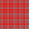
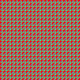
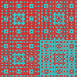
I’d like produce something similar in color, but there’s a slight problem: we don’t have a finite number of elements. To get around this, we’ll have to take our tables mod an integer. In the HSV color space, colors are cyclic just like the integers mod n. This actually has an additional appealing feature: two colors with similar hues are “near” in a similar way to the underlying numbers. Then, the entry-to-color mapping can just be given as
k \mapsto HSV \left({2\pi k \over n}, 100\%, 100\% \right)
In this mapping, for n = 2, zero goes to red and one goes to cyan. The following is a 100x100 image of the multiplication table of \oplus_\text{Zeck} from zero to ninety-nine.
Anima Moduli
This table can by animated by gathering various n into an animation and incrementing n every frame. Before applying this technique to an error table, it’d be prudent to apply it to standard addition and multiplication tables first.

Both images appear to zoom in as the animation progresses. Unsurprisingly, addition produces diagonal stripes, along which the sum is the same. Multiplication produces a squarish pattern (with somewhat appealing moirés).
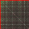
Tables for \odot_\text{Zeck} and \oplus_\text{Zeck} should resemble the table to the right, since their definition relies on it.
Indeed, the zooming is present in both tables. At later frames, both tables share the same “square rainbow” pattern, but the error table is closer. Though both tables appear to have a repeating pattern, the blocks in the error table are still irregularly shaped, as in the mod 2 case.
The error table also demonstrates (for a given modulus) how much the series differs from a geometric series. We know there will always be an error since, while Fibonacci numbers grow on the order of O(\varphi^n), the ratio between place values is only φ in the limit.
Other Error Tables
These operations can can also be defined in terms of any other series expansion (i.e., integral system). Rather than showing both of the multiplication and error tables, I will elect to show only the latter. The error table is more fundamental since the table for \odot can be constructed from it and the normal multiplication table.
The error tables for some of the previously-discussed generalizations of the Fibonacci numbers are presented below.
Pell, Jacobsthal

Of the two tables, the Pell table looks more similar to the Fibonacci one. Meanwhile, the Jacobsthal table has frames which are significantly redder than the either surrounding it. These occur on frames for which n is a power of 2, which is a root of the recurrence polynomial.
n-nacci
Compared to the Fibonacci image, the size of the square pattern in the Tribonacci and Tetranacci images is larger. Higher orders of Fibonacci recurrences approach binary, so in the limit, the pattern disappears, as if the tiny red corner in the upper-left is all that remains.
Other
Of course, integral systems are not limited to linear recurrences, and tables can also be produced that correspond to other integer sequences. For example, the factorials produce distinct patterns at certain frames. The Catalan numbers (which are their own recurrence) mod two seem to make a fractal carpet. To prevent the page from getting bloated, these frames are presented in isolation.
Additional tables which I find interesting are:
Closing
Even if not particularly useful, I enjoy the emergent behavior apparent in the tables. Even for typical multiplication, this visualization technique shows regular patterns which appear to “grow”. Meanwhile, the sequence products frequently produce a pattern that either repeats, or is composed of many similar elements.
The project that I used to render the images can be found here. I didn’t put much thought into command line arguments, nor did I build in many features. As an executable, it should be completely serviceable to generate error tables based on recurrence relations; the GHCi REPL can be used for more sophisticated sequences.
Bad Visualization
My first attempt to map integers to colors was to consider its prime factorization. The largest number in the factorization was related to the hue, and the number of terms in the factorization was related to the saturation. Results were not great.
Bad Filesizes
While I rendered these animations as GIFs, I also attempted to convert some of them to MP4s in hopes of shrinking the filesize. However, this is a use case where the MP4 is larger than the GIF, at least without compromising on resolution. This is a case when space-compression beats ill-suited time-compression.
