Counting in 2D, Part 1: Lines, Leaves, and Sand

An introduction to two-dimensional counting using polynomials of two variables.

Previously, I’ve written about positional systems and so-called “polynomial counting”. Basically, this generalizes familiar integer bases like two and ten into less familiar irrational ones like the golden ratio. However, all systems I presented have something in common: they all use polynomials of a single variable. Does it make sense to count in two variables?

Preliminaries

Before proceeding, I’ll summarize some desired characteristics of polynomials which can be used as carries in positional systems.

Carry polynomials must be nonpositive when evaluated at 1 (otherwise the digital root of an expansion is unbounded). Moreover, to make things easier, either:

• All coefficients have the same sign but one, which has a much larger magnitude than the rest (and forces the digital root condition)
  • These are explicit irrational carries
• They are monic (have leading coefficient 1) and the remaining coefficients are all negative and monotonically increase toward 0 after the second coefficient (0’s are allowed anywhere)
  • These are implicit irrational carries

In previous systems, it was discovered that implicit carries can be multiplied, typically by cylotomic polynomials, to obtain explicit rules for larger numerals.

A Game of Che…ckers

Conway’s checkers is a game played by attempting to advance game pieces to the furthest extent beyond a line. A piece can only be moved by jumping it horizontally or vertically over others, which removes them from play. Squinting hard enough, in one dimension, this is similar to how in phinary, a “1” in an expansion can jump over an adjacent “1” to its left.

\begin{array}{} \bullet \\ \hline \bullet \\ \hline \vphantom{\bullet} \end{array} \huge⤸ \normalsize ~\longrightarrow~ \begin{array}{} \vphantom{\bullet} \\ \hline \vphantom{\bullet} \\ \hline \bullet \end{array} \quad \iff \quad 0\textcolor{red}{11} = \textcolor{red}{1}00

In fact, it is exactly the same. The best solution of the game relies on a geometric series in φ, as seen in this video by Numberphile.

Pairs of Checkers

To actually take phinary and systems like it from 1D to 2D, we really just need a carry rule that respects the second dimension. To do this, we use a new variable y and invent a carry rule based on it.

The smallest way to extend our one-dimensional string of digits is do just introduce a second string. Based on this, my intuition was to replace the standard hop with the movement of a knight in chess.

\begin{gather*} \begin{array}{c|c} \bullet & \phantom{\bullet} \\ \hline \bullet \\ \hline \vphantom{\bullet} \end{array} ~\longrightarrow~ \begin{array}{c|c} \phantom{\bullet} & \phantom{\bullet} \\ \hline \\ \hline & \bullet \end{array} ~~ \iff ~~ \left. \begin{array}{} 0\textcolor{red}{11}_x \\ 000_y \end{array} \right] = \left. \begin{array}{} 000_x \\ \textcolor{red}{1}00_y \end{array} \right ] \\ \\ y^2 = x + 1,~ x^2 = y + 1 \end{gather*}

This looks good on the surface, but it turns out that the polynomials aren’t sufficiently intertwined. Since each variable is a function of the other, they can easily be coaxed into a single polynomial:

y = x^2 - 1 \longrightarrow y^2 = (x^2 - 1)^2 = x + 1 \\[6pt] x^4 - 2x^2 + 1 = x + 1 \\ x^3 - 2x - 1 = 0 \\ (x + 1)(x^2 - x - 1) = 0

The same argument applies symmetrically for y. One of the resultant polynomials is the minimal polynomial of φ, so the prospective 2D system reduces back to standard phinary.

There are additional problems with this “pairs of strings” model. For example, terms like xy never appear, and there is no way to represent them by just using two strings. Also, both sequences have a ones’ place, but should agree that x^0 = y^0 = 1.

Building the Plane

If it is the case that both powers of variables should share the one’s digit, then why not join the two strings there? In other words, for each variable, we think of a line with a distinguished point for zero. We then match the distinguished points together. Thus, instead of a point separator between positive and negative powers, the radix point is now a pair of lines that share a vertex. From this pair of lines, according to Euclid, we can make a plane.

\begin{array}{|c} \hline f & d & a \\ e & b \\ c \end{array} \begin{matrix} ~\equiv~ ax^2 + bxy + cy^2 + dx + ey + f, \\ \text{the general form of a conic} \end{matrix}

Since the horizontal and vertical correspond with the x and y appearing in polynomials, it may be easy to confuse this with the x- and y-axes of the typical Cartesian plane. The key differences here are that these are discrete (two-dimensional) strings, rather than a continuous plane, and along each point, there exists a cell in which an integer value lives.

An Arithmetical Aside

Expressed in this way, it is very simple to compute the sum of two polynomials. Just like in the 1D system, we can align the one’s places, add them together term-by-term, then apply carry rules. With luck, this produces a canonical form.

It should also be possible to multiply two polynomials together. In a single variable, multiplication is a somewhat involved 1D convolution. In two, it is naturally 2D convolution, an operation typically encountered in image processing and signal analysis. I won’t bother building up an intuition for this, since it won’t be relevant to discussion.

Even if multiplication is difficult, division is always harder. In polynomials of a single variable, we can do synthetic (or long) division. Notationally, we work in the direction that the digits do not extend (i.e., downward). With 2D numbers, we have digits in both dimensions. Fortunately, computer algebra systems can divide and factor polynomials of two variables reasonably quickly, so this point is moot if we allow ourselves to use one.

1, 2, 3, Takeoff

Where should we start in a world of planar numbers? Well, we want to assign an integer to a polynomial with extent in both x and y. The simplest way to do this is by letting n = x + y: when the one’s place has a magnitude of n, it flows into x and y.

If n = 1, then the sum of coefficients is skewed toward the LHS, and the digital root is unbounded. We had a similar restriction in one dimension. Therefore, let n = 2. The expansions of the powers of 2 are:

\begin{matrix} &&\text{Carry:}&\begin{array}{|c} \hline -2 & 1 \\ 1 \end{array}\\ 1 & 2 & ... & 4 & ... & 8 \\ \begin{array}{|c} \hline 1 \end{array} & \begin{array}{|c} \hline 0 & 1 \\ 1 \end{array} & ... & \begin{array}{|c} \hline 0 & 2 \\ 2 \end{array} & ... & \begin{array}{|c} \hline 0 & 4 \\ 4 \end{array} \\ \\ &&& \begin{array}{|c} \hline 0 & 0 & 1 \\ 0 & 0 & 1 \\ 1 & 1 \end{array} & ... & \begin{array}{|c} \hline 0 & 0 & 2 \\ 0 & 0 & 2 \\ 2 & 2 \end{array} \\ \\ &&&&& \begin{array}{|c} \hline 0 & 0 & 0 & 1 \\ 0 & 0 & 1 & 1 \\ 0 & 1 & 0 & 1 \\ 1 & 1 & 1 \end{array} \end{matrix}

The final entry of each column is achieved by applying the carry enough times, reducing all digits to “0”s and “1”s. In doing so, the typical binary expansion is visible along first row and column, albeit reversed. This is always the case, since when the carry is restricted to a single dimension (i.e., let y = 0), we get the 1D binary carry. More visually, there is no mechanism for the carry to disturb the column and row by spreading either left or up. I’ll call this system dibinary, since it is binary across two variables.

An additional property of this system is that the number of “1”s that appear in the expansion is equal to the number itself. These two properties make it a sort of hybrid between unary and binary, bridging their binary expansion and its Hamming weight.

This notation is very heavy, but fortunately lends itself well to visualization. Each integer’s expansion is more or less an image, so we can arrange each as frames in a video:

Starting at the expansion of twelve, the terms extend past the first column and row. It instead grows faster along the diagonal, along which larger triangles appear when counting to higher and higher integers. Meanwhile, lower degrees (toward the upper left) appear to be slightly less predictable.

Higher n

By incrementing n, the expansions of numbers shrink exponentially, and simply incrementing is not fast enough. Fortunately, this is a simple enough system that we can scalar-multiply base expansions, then assiduously apply the carry. Ascending the powers of n in this manner for the carries where n = 3 and 4:

x + y = 3

x + y = 4

Yellow corresponds to the highest allowed numeral, n - 1. It seems like the lower-right grows much rounder as n increases. However, neither appears to have an emergent pattern as dibinary did.

You might be familiar with the way hexadecimal is a more compact version of binary. For example,

\textcolor{red}{1}\textcolor{blue}{2}_{16} = \textcolor{red}{0001}\textcolor{blue}{0010}_{2}

because both one hexadecimal digit and four binary digits range over zero to fifteen. Consequently, by grouping group m digits of an expansion in base b, one can easily convert to base b^m.

If such a procedure still exists in 2D, applying it somehow destroys the pattern in the n = 2 case, as the quaternary system is very chaotic.

Carry Curves

Since the carry is a polynomial in both x and y, it lends itself to interpretation as an algebraic curve. Taking x or y to higher powers will dilate expansions along that axis.

The carry is not the only curve which exists in a system, as each integer is also a polynomial unto itself. Adding a constant term will not change anything unless it causes carries to occur. Starting at the carry digit, some of the incremented curves made by the carry x + y = 2 are shown below.

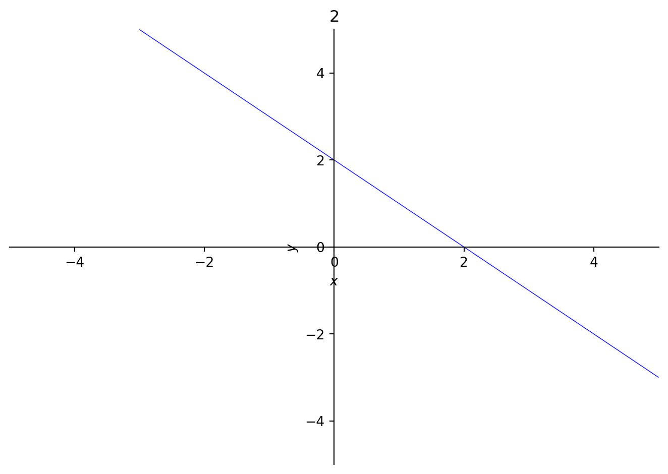
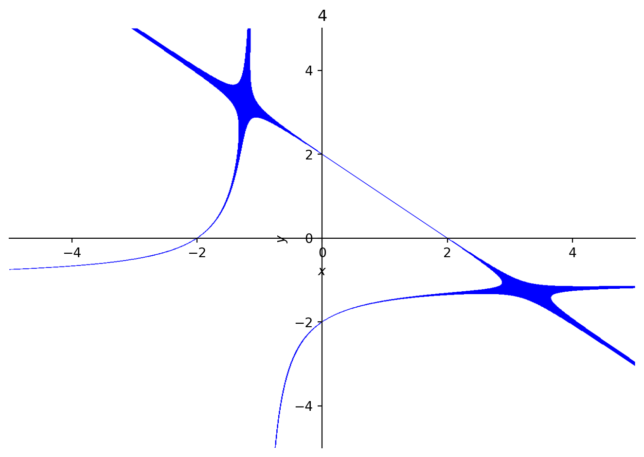
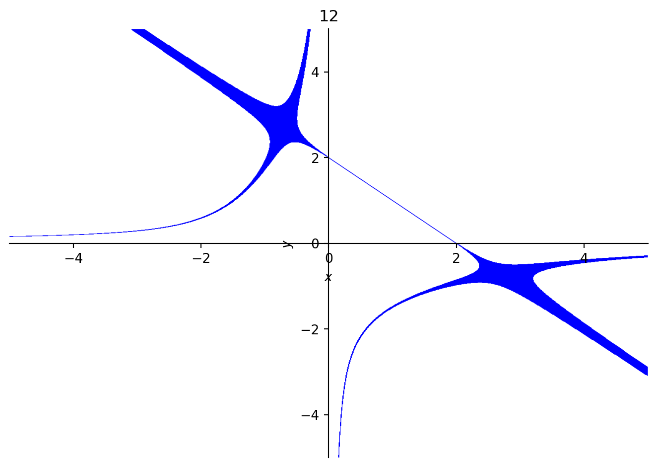
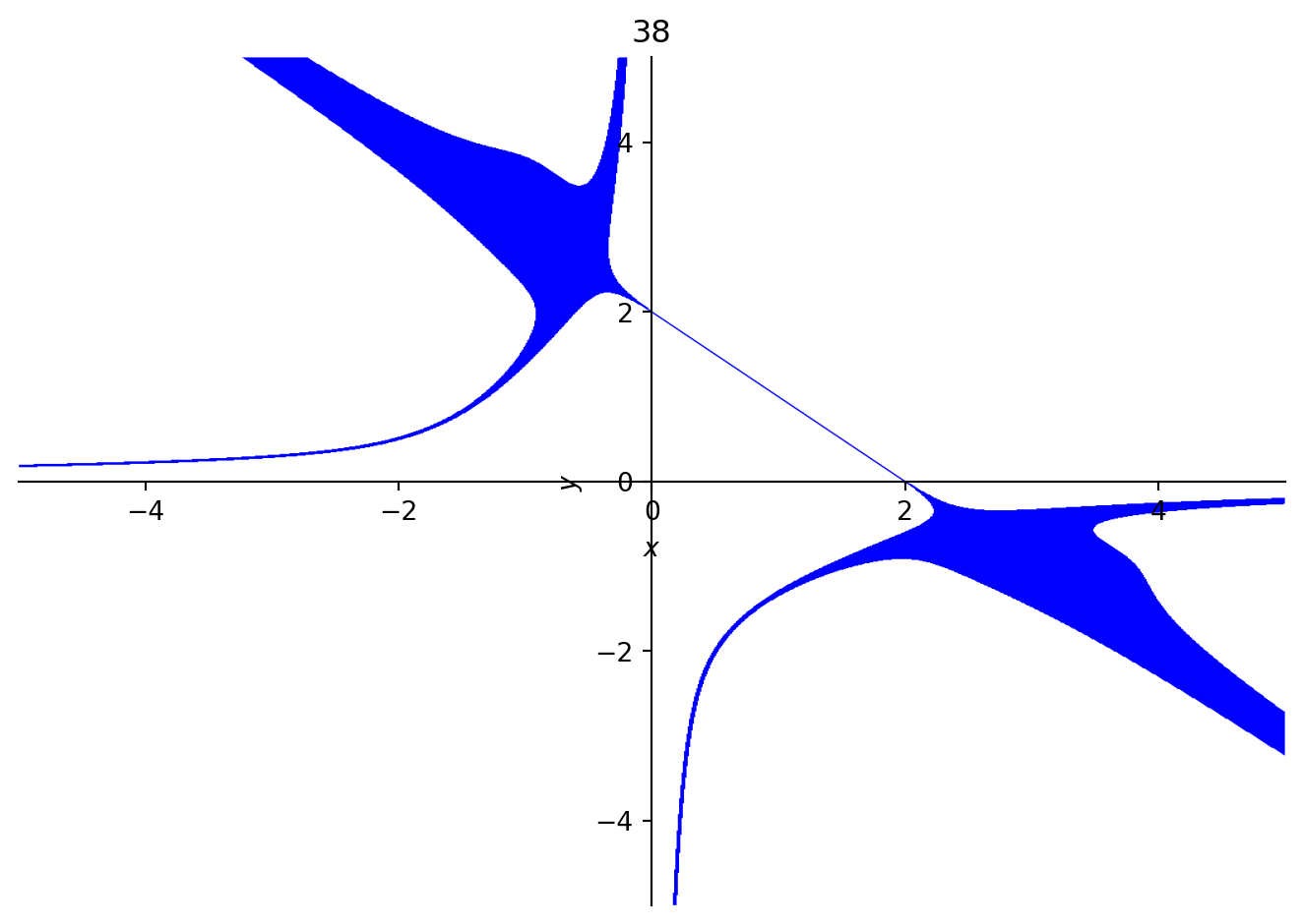
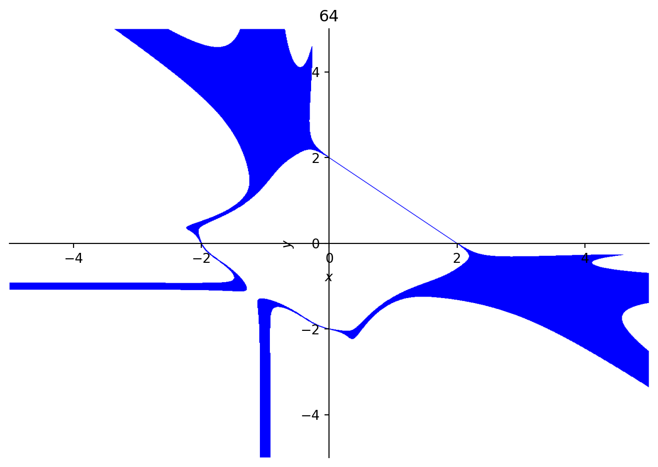
In each of these figures, the line is the curve which corresponds to the carry polynomial. Along with it, while counting, additional shapes like hyperbolae seem to appear and disappear, only to be replaced with higher-order curves. These higher order curves can be difficult to graph, so they show up as thicker lines. At sixty-four, it appears as though the reflection of the carry across the origin (the curve x + y = -2) “wants” to appear.

The continued presence of the original carry curve in larger integers suggests that the points it passes through are important. This curve happens to intersect with the x and y axes, which we can interpret as the “base” with respect to a single variable. For dibinary, these are the aforementioned “typical binary expansions”. We can also evaluate the polynomial at (x, y) = (1, 1), a point on the carry curve, to compute its digital root, which is also equal to the integer it represents. This underlies a key difference from the 1D case. 1D systems are special because the carry can be equated with a base (or bases), which is a discrete, zero-dimensional point (one dimension less) on a number line. In higher dimensions, all points on the carry curve (or hypersurface) are “bases” we can plug in to test that an expansion is valid. This makes naming much harder, since there are no preferred numbers to represent the system, like the golden ratio does with phinary.

Casting the Line

We may want to extend the “unary” property to other carries. To do this, we construct a curve which passes through (1, 1).

Lines of the form (n - 1)x + y = n trivially satisfy this relationship. Further, while the digits along the y column will be expansions of base n, those along x will be in base n / (n - 1).

For example, for n = 3

\begin{matrix} &&&\text{Carry:}& \begin{array}{|c} \hline -3 & 2 \\ 1 \end{array}\\ 1 & ... & 3 & ... & 6 & ... & 9 \\ \begin{array}{|c} \hline 1 \end{array} & ... & \begin{array}{|c} \hline 0 & 2 \\ 1 \end{array} & ... & \begin{array}{|c} \hline 0 & 4 \\ 2 \end{array} & ... & \begin{array}{|c} \hline 0 & 6 \\ 3 \end{array} \\ \\ &&&& \begin{array}{|c} \hline 0 & 1 & 2 \\ 2 & 1 \end{array} & ... & \begin{array}{|c} \hline 0 & 3 & 2 \\ 3 & 1 \end{array} \\ \\ &&&&&& \begin{array}{|c} \hline 0 & 0 & 1 & 2 \\ 0 & 1 & 0 & 2 \\ 1 & 1 & 1 \end{array} \end{matrix}

The expansion in the y column looks trivially correct, since y^2 = 9 when x = 0. We can check the base of the expansion of nine (“2100”) by factoring a polynomial:

\displaystyle 2 x^{3} + x^{2} - 9 = \left(2 x - 3\right) \left(x^{2} + 2 x + 3\right)

The linear polynomial has 3/2 as a root, while the quadratic one has only complex roots.

Naturally, these expansions work symmetrically by considering y to have the n - 1 coefficient instead of x. This transposes the carry (and hence the expansion).

Slanted Counting

For good measure, let’s see what it looks like when we count in the n = 3 and n = 4 cases.

2x + y = 3

3x + y = 4

The pattern produced is similar to the one from dibinary. However, the triangular pattern no longer grows all at once, and instead, the bottom leads the top. Meanwhile, the disordered part in the upper left of the expansion appears to grow larger as n increases, not to mention that it contains many artifacts from smaller colors.

The slope of the pattern is 1 / (n - 1), since this is the ratio of growth between x and y. As n grows, the diagonal pattern gets thinner and takes longer to show up. This is because the size of the alphabet causing expansions to shrink geometrically, while the digital root is always increasing arithmetically. The binary alphabet is the smallest possible, so the minimal shrinkage is in dibinary.

Incremented Curves

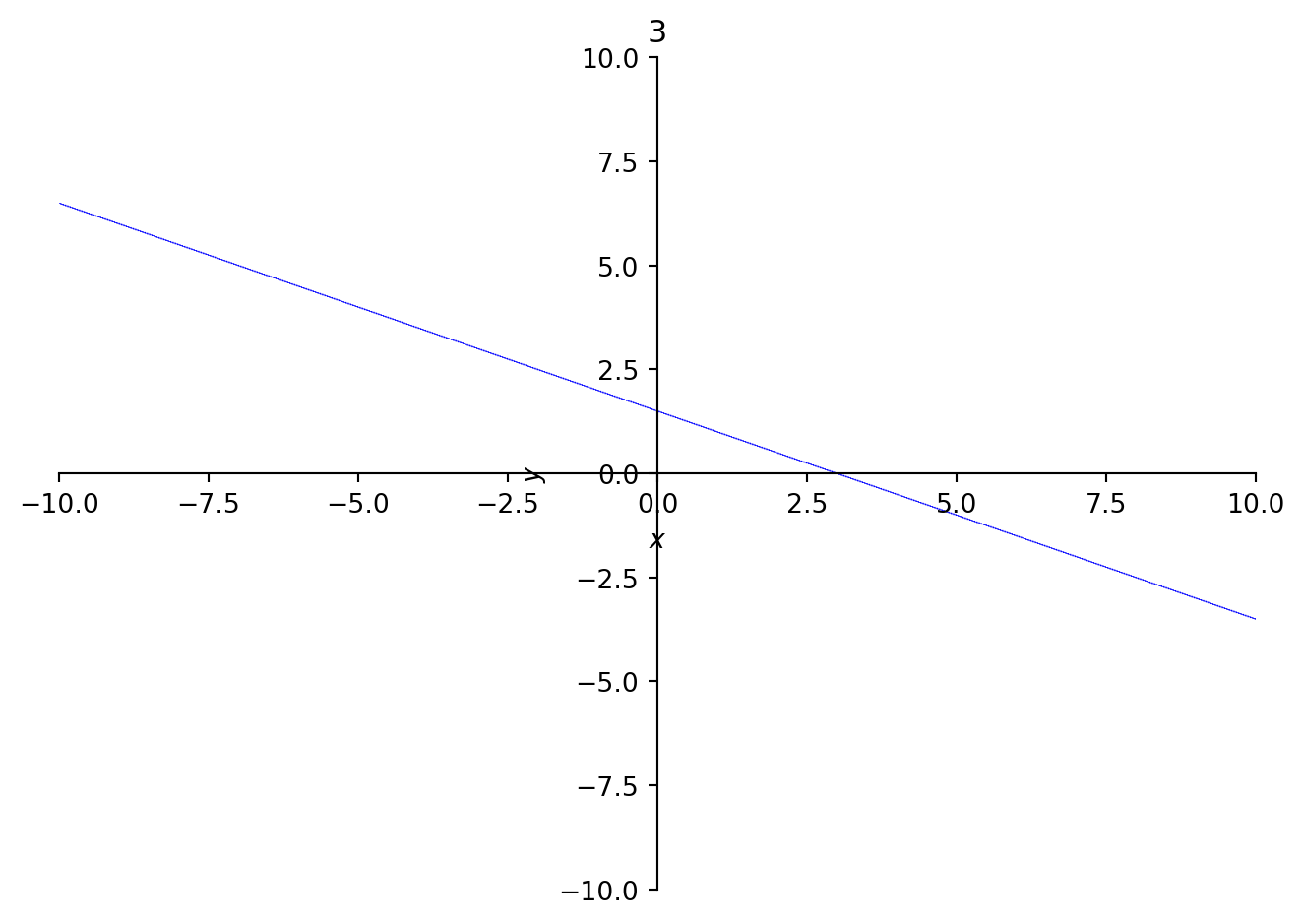
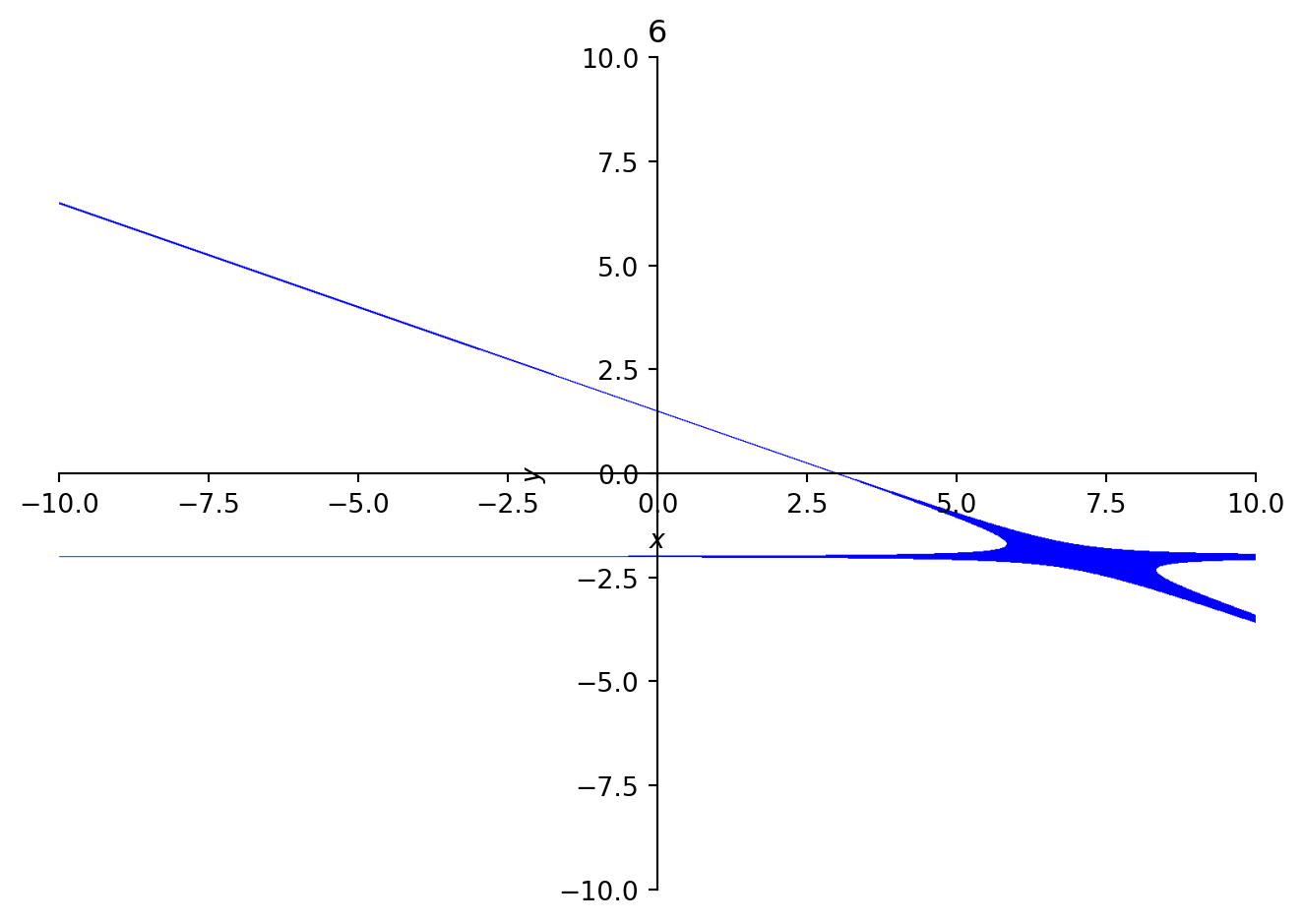
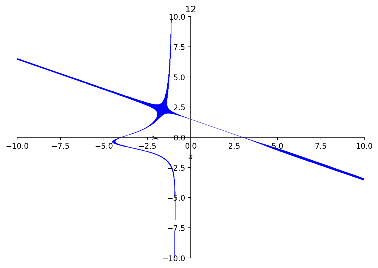
Below are some incremented curves for n = 3. These curves show an interesting phenomenon: an extra line is present in in the expansion of six. This line turns into a spike at twelve, then at fifteen, it seems to grow to encompass the point at infinity.

Leaves in the Mirror

Algebraic curves are not my forte. Still, we can very briefly look at some classical examples from the perspective of carries.

Quadratic Curves

Unfortunately, the most common quadratic curves are largely uninteresting. Briefly, here are some comments about some the simplest cases:

• Unit circle (x^2 + y^2 - 1 = 0) and hyperbola (\pm x^2 \mp y^2 - 1 = 0)
  • The sum of coefficients is positive, which means that expansions are unbounded.
  • Alternatively, coefficients are of an improper form, since one positive coefficient does not outweigh all remaining negative coefficients.
  • The curve as a function in x and y can be written in simpler terms, i.e., F(x, y) = G(x^2, y^2)
• Hyperbola (xy \pm 1 = 0)
  • The curve is a function of only xy, i.e., F(x, y) = P(xy), so the curve degenerates to one-dimensional unary.
• Parabolae (y = \pm x^2,~ x = \pm y^2)
  • One coefficient does not outweigh the other.
  • The system degenerates to a single dimeension due to the fact that either y is a polynomial in x or vice versa

Other polynomials in x and y may produce rotations or dilations of these curves, but the key fact is that this interpretation is secondary. What truly matters is that one cell affects relatively close cells in a certain way.

Higher-Order Curves

All unit Fermat curves x^n + y^n = 1 are not suitable as carries, since their digital root is unbounded. Scaling up the curve, for example to x^n + y^n = 2, will just degenerate back to the previous examples with lines, but spaced out by zeros between entries.

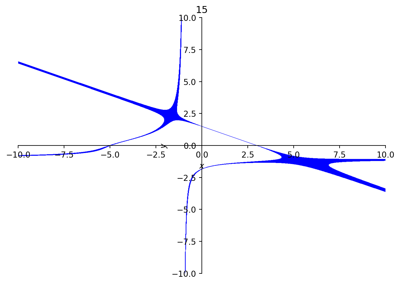
The folium of Descartes is another classical curve that played a role in the development of calculus, described by the equation:

\begin{gather*} x^3 + y^3 - 3axy = 0 \\ \\ \begin{array}{|c} \hline 0 & 0 & 0 & 1 \\ 0 & -3a \\ 0 & \\ 1 \end{array} \end{gather*}

As written above, the position of the 3a term may be confusing. As the negative term in an explicit carry, we must place it atop the digit we are carrying, meaning that expansions will propagate toward negative powers of x and y as well as positive. While the shape of the curve is different from an ordinary line, the coefficients are arranged too similarly; for a = 2/3 (so the curve passes through the point (1, 1)) incrementing appears as:

\begin{gather*}2: &\begin{array}{c|cc}0 & 0 & 0 & 1 \\ \hline 0 & 0 & 0 & 0 \\ 0 & 0 & 0 & 0 \\ 1 & 0 & 0 & 0 \\ \end{array}\\\\ \\ 4: &\begin{array}{cc|cccc}0 & 0 & 0 & 0 & 0 & 0 & 1 \\ 0 & 0 & 0 & 0 & 0 & 0 & 0 \\ \hline 0 & 0 & 0 & 0 & 0 & 1 & 0 \\ 0 & 0 & 0 & 0 & 0 & 0 & 0 \\ 0 & 0 & 0 & 0 & 0 & 0 & 0 \\ 0 & 0 & 1 & 0 & 0 & 0 & 0 \\ 1 & 0 & 0 & 0 & 0 & 0 & 0 \\ \end{array}\\\end{gather*}

Clearly, this also tends back toward dibinary, but with the yellow digits spaced out more.

Laplace’s Sandstorm

As stated previously, polynomials naturally multiply by convolution. In the context of this operation, the discrete 2D Laplacian is frequently used While commonly presented as a matrix, it has very little to do with the machinery of linear algebra which normally empowers matrices.

\begin{gather*} \begin{bmatrix} 0 & 1 & 0 \\ 1 & -4 & 1 \\ 0 & 1 & 0 \end{bmatrix} ~\implies~ \begin{array}{c|cc} & 1 & \\ \hline 1 & -4 & 1 \\ & 1 \end{array} \\ \\ x + x^{-1} + y + y^{-1} - 4 = 0 \\ x + xy^2 + y + yx^2 - 4xy = 0 \end{gather*}

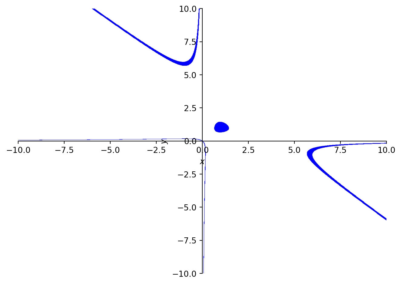
From the above, it is clear that this is a cubic curve. Aside from the trivial solution x = y = 0 (which obviously also satisfies x = y), the curve made by the carry does not intersect either axis. There is an additional isolated point at (1, 1), implying some is in unary-ness this system. If we make it a carry, then the first few powers of 4 are

\begin{matrix} 1 & ... & 4 & ... & 16 \\ \begin{array}{|c} \hline 1 \end{array} & ... & \begin{array}{c|cc} 0 & 1 & 0 \\ \hline 1 & 0 & 1 \\ 0 & 1 & \end{array} & ... & \begin{array}{c|cc} 0 & 4 & 0 \\ \hline 4 & 0 & 4 \\ 0 & 4 & \end{array} \\ \\ &&&& \begin{array}{cc|cc} & & 1 \\ & 2 & 0 & 2 \\ \hline 1 & 0 & 4 & 0 & 1 \\ & 2 & 0 & 2 \\ & & 1 \end{array} \\ \\ &&&& \begin{array}{cc|cc} & & 1 \\ & 2 & 1 & 2 \\ \hline 1 & 1 & 0 & 1 & 1 \\ & 2 & 1 & 2 \\ & & 1 \end{array} \end{matrix}

As the negative (and largest) term, we carry at the “4” entry, as shown above. Terms progress along lower and higher powers of x and y. However, rather than just rightward propagation interfering with downward propagation (and vice versa), all directions can interfere with each other.

This system can be interpreted more naturally as a sandpile. As a cellular automaton, it is rather popular as a coding challenge (video by The Coding Train), and when the grid is finite, certain subsets of all possible elements form finite groups under addition (video by Numberphile). These videos discuss toppling the initial value, but do not point out the analogy to polynomial expansions.

The shapes produced by this pattern are well-known, with larger numbers appearing as fractals. Generally, the expansions are enclosed within a circle, with shrinking triangular looking sections. This is eerily similar to the same shrinking triangles which appear in other unary-like carries.

Closing

All of the 2D carries presented here are explicit carries. Unlike phinary, they have no additional rules hidden in mutliples of the carry. It seems to be the case that implicit carries in two variables can be found by selecting a cyclotomic polynomial (in x, y, and x + y) and computing an explicit carry by multiplying it with another polynomial. Some of my investigations into this topic are available here.

I should also mention that my notational inspiration for arranging digits things in a 2D array is Norman Wildberger’s variable-free approach to “bipolynumbers”, a term he uses to refer to polynomials of two variables.

Just as learning to count on polynomials in a single variable opens up a world of possibilities, learning to count on those in two variables is a perplexing topic that is worth exploring.